AWS Database Blog
Characterizing SQL*Net latency in your application for Oracle Database@AWS migrations
Oracle Database@AWS (ODB@AWS) is an offering that enables you to access Oracle Exadata infrastructure managed by Oracle Cloud Infrastructure (OCI) inside AWS data centers. ODB@AWS delivers low-latency network connectivity to AWS services like Amazon Elastic Compute Cloud (Amazon EC2), Amazon Elastic Container Service (Amazon ECS), and Amazon Elastic Kubernetes Service (Amazon EKS) running in an Amazon Virtual Private Cloud (Amazon VPC). SQL*Net traffic between application hosts and Exadata traverses ODB Peering, which routes traffic privately between an Amazon VPC and an ODB network.
In this post, we present a methodology to help you prepare your database and application workload for migration to ODB@AWS. The methodology helps you assess whether your on-premises workload is sensitive to SQLNet latency and understand the impact of any additional SQLNet latency introduced by the ODB@AWS multi-cloud architecture. We also discuss connectivity and deployment considerations for ODB@AWS candidates.
Why it is important to assess SQL*Net latency for ODB@AWS migrations
When migrating to ODB@AWS, an important question is whether your workload exhibits sensitivity to potentially increased SQLNet latency. Workloads with SQL statements that are extremely quick (sub-millisecond database processing time), frequent (thousands of executions per second), and concentrated (driven by a small number of sessions) are potentially sensitive to increases of even hundreds of microseconds of SQLNet round-trip latency, directly affecting application performance. The method presented in this post will show you how to determine whether your application workload has these three characteristics, and if so, quantify the potential impact before you migrate.
One maxim remains forever true: lower-latency client networks cannot negatively impact application performance, but they might not improve performance. Oracle has published guidance on reducing SQL*Net round trips for decades. Stored procedures, array fetch operations, and bulk processing move work server-side or batch it, reducing the number of client-server round trips. As Oracle’s own Net Services documentation states:
“Tuning your application to reduce the number of round trips across the network is the best way to improve your network performance.”
However, if your application has modules that remain acutely sensitive to SQL*Net latency even after such optimizations, this method will help you identify and quantify that sensitivity before migration.
Methodology overview
The method uses standard Oracle performance tooling (Automatic Workload Repository (AWR), Active Session History, and SQL Trace) and consists of three phases:
- Phase 1: AWR screening to identify candidate SQL statements.
- Phase 2: Validate candidate SQL statements from Phase 1 with SQL Execution Session Density (SESD).
- Phase 3: Characterize SQL*Net latency sensitivity through SQL Trace and Client Request Elapsed Time (CRET) analysis.
Methodology deep dive
Introducing the Client Request Elapsed Time (CRET)
This methodology takes a novel approach by centering on an Oracle idle wait event as the primary instrument for assessing SQLNet latency sensitivity. The specific idle wait is SQLNet message from client (SNMFC). Two consecutive SNMFC waits bracket what we refer to as a Client Request Elapsed Time (CRET) event.
Every SQL request from a client application to a database instance through SQL*Net follows a three-stage timeline:
- Client Time + Client-to-Server Network Time: The client application processes the previous result (or remains idle), then sends the next SQL request through SQL*Net to the database server. Client Time includes computation tasks, web-tier interaction, or idle time such as a GUI application waiting for human input. During this entire stage, the database session is waiting in a SNMFC wait for the next request to arrive.
- Database Processing Time: The database server receives the request, processes it, and prepares the response.
- Server-to-Client Network Time: The database server sends the result set or completion code to the client application through SQL*Net. Immediately after sending, the database session returns to a SNMFC wait.
The sum of stages 1 and 3 constitutes Non-Database Time. Stage 2 is entirely in-database processing and has nothing to do with SQL*Net client network latency.
CRET = Database Time + Client Time + SQL*Net RTT
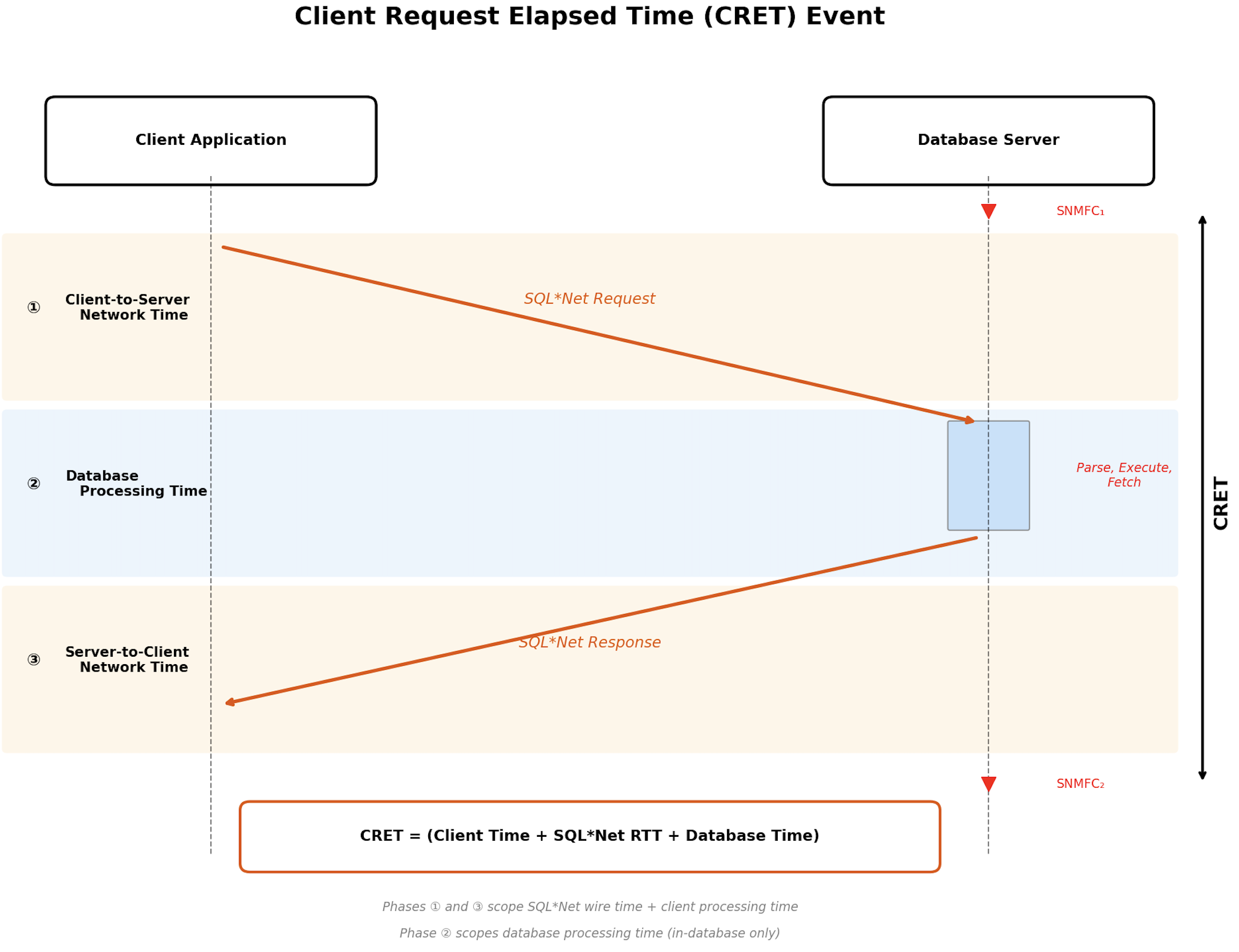
Figure 1: Client request timeline, where two consecutive message from client waits bracket one CRET event
Introducing the CRET method
The following is a deep dive on the CRET Method consisting of three sections: Phase 1 (AWR Screening), Phase 2 (SQL Execution Session Density), and Phase 3 (SQL Trace and CRET Analysis).
Phase 1: AWR screening (identify candidate SQL statements)
Start with an AWR report that spans a period of suspected latency-sensitive application activity and note the AWR elapsed time from the header. For example, the following graphic shows an AWR header section for a report that spans 30 minutes.

Figure 2: AWR report header showing a 30-minute snapshot window
The goal of the screening is to identify SQL statements that are frequent and quick, meaning thousands of executions per second with microsecond-level database processing time. Navigate to the SQL Ordered by Executions section and for each top SQL statement calculate the executions per second (total executions divided by AWR elapsed time in seconds) and the average database processing time (total elapsed time divided by execution count). SQL statements with sub-millisecond database processing time combined with thousands of executions per second are latency-sensitivity candidates. SQL statements with multiple-millisecond processing time are generally tolerant of additional SQL*Net latency because the database processing time per execution dwarfs the added network time.
An example of Phase 1 screening
In this real-world example, an AWR report spanning 360 minutes (21,600 seconds) contains a SQL Ordered by Executions section. The screenshot below shows the top five rows from that section, and the table that follows shows the Phase 1 analysis of each.

Figure 3: AWR SQL ordered by executions section listing the top five SQL statements by execution count
| SQL_ID | Elapsed Time (s) | Executions | Exec/Sec | Avg DB Time | Assessment |
| …f243rp | 10,966 | 112,622,398 | 5,214/sec | 97 µs | Candidate. Proceed to Phase 2. |
| …t4xvug | 9,809 | 97,577,695 | 4,517/sec | 101 µs | Candidate. Proceed to Phase 2. |
| …r5tj7z | 15,302 | 57,889,149 | 2,680/sec | 264 µs | Candidate. Proceed to Phase 2. |
| …r8qyvu | 13,509 | 40,966,821 | 1,897/sec | 330 µs | Candidate. Proceed to Phase 2. |
| …9uyp0z | 18,471 | 24,081,444 | 1,115/sec | 767 µs | Possible candidate. Approaching millisecond DB processing time but still sub-millisecond. Proceed to Phase 2. |
Phase 2: SQL Execution Session Density (SESD)
Phase 1 uses AWR to identify candidate SQL statements that are quick and frequent. However, the execution counts in the SQL Ordered by Executions section are instance-wide aggregates, summed across all sessions. AWR does not tell you whether those executions come from one session or a thousand. Before proceeding to Phase 3, make sure the candidate SQL statement is being executed by one or very few sessions.
The concept is straightforward. If a SQL statement requires 100μs of database processing time per execution, a single session executing it 10,000 times per second is indistinguishable in AWR from 100 sessions each executing it 100 times per second. Only the former is latency-sensitive: concentrated executions from few sessions indicate High SESD and warrant Phase 3 analysis, while executions distributed across many sessions indicate Low SESD and Phase 3 is not needed.
SESD can be determined by querying Active Session History for distinct session counts observed executing the SQL_ID, by querying the USERS_EXECUTING column in V$SQL, or by consulting the application owner who understands how the application works. High SESD warrants Phase 3 analysis. Low SESD does not.
SQL Execution Session Density – deep dive
Consider SQL_ID 52cn24qf243rp from the Phase 1 AWR above which executed 5,214 times per second with 97μs average database processing time. Suppose SESD assessment reveals this SQL_ID is executed by only 5 sessions. Each session would sustain approximately 1,043 executions per second, yielding an execution budget of approximately 959μs per CRET cycle (1,043 × 959μs = 1,000,000μs = 1 second). With a low value (959us) for the CRET cycle time, changes in SQL*Net latency could have a large impact on relative performance and that is what Phase 3 will help us evaluate. This SQL statement would be a prime candidate for Phase 3 analysis. On the contrary, if those same 5,214 executions per second were spread across 200 sessions, each session could execute it roughly every 38 milliseconds and therefore would not warrant Phase 3 analysis.
Phase 3: SQL Trace + CRET analysis
At this point in the assessment, Phase 1 screening has identified a SQL statement that is quick and frequent, and Phase 2 SESD analysis has confirmed that its executions are concentrated in very few sessions. What remains is to trace one of those sessions and quantify the actual latency sensitivity through CRET event analysis.
Enabling SQL Trace
Identify a session actively executing the candidate SQL statement and enable trace with wait events:
Allow sufficient trace duration to capture a representative sample of executions. When tracing is complete, disable:
The CRET paragraph: A real-world example
The following graphic shows a real CRET paragraph from a SQL Trace file. Two consecutive SNMFC waits (highlighted in red) bracket the paragraph.
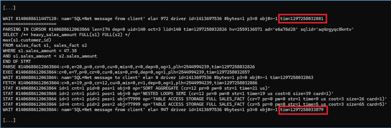
Figure 4: SQL Trace excerpt with two consecutive message from client waits highlighted
The CRET duration is the time delta between the two SNMFC tim= values, calculated as 1,297,258,033,879 minus 1,297,258,032,801, which equals 1,078µs. The closing SNMFC ela= value (947µs) accounts for the Non-Database Time in this CRET cycle. Subtracting Non-Database Time from the CRET duration gives Database Time, calculated as 1,078 minus 947, which equals 131µs.
The CRET analysis tool
The following four one-liner AWK commands comprise a CRET analysis tool. Each accepts the name of a trace file to process as the first argument to the script and requires gawk(1). No Oracle client software is required as the one-liners operate directly on the SQL Trace file. The four one-liners report:
- One-liner 1 — CRET summary: Total elapsed time, CRET count, and CRET rate (CRETs/sec).
- One-liner 2 — SNMFC elapsed percentiles: Non-Database Time distribution (Min, P50, P90, P99, Max).
- One-liner 3 — CRET elapsed percentiles: Complete round-trip time distribution (Min, P50, P90, P99, Max).
- One-liner 4 — Latency impact projection: Projected runtime increase for +100μs, +150μs, and +200μs added SQL*Net RTT.
One-liner 1 — CRET summary
One-liner 2 — SNMFC elapsed percentiles
One-liner 3 — CRET elapsed percentiles
One-liner 4 — Latency impact projection
Worked examples: CRET analysis output
The following screenshot demonstrates the four one-liner commands applied to two contrasting trace files, each with 10,000 CRET events, that differ entirely in client-side execution pattern. One is a tight loop, the other includes significant client-side processing delays between requests. The one-liner output quantifies the latency sensitivity of each pattern.
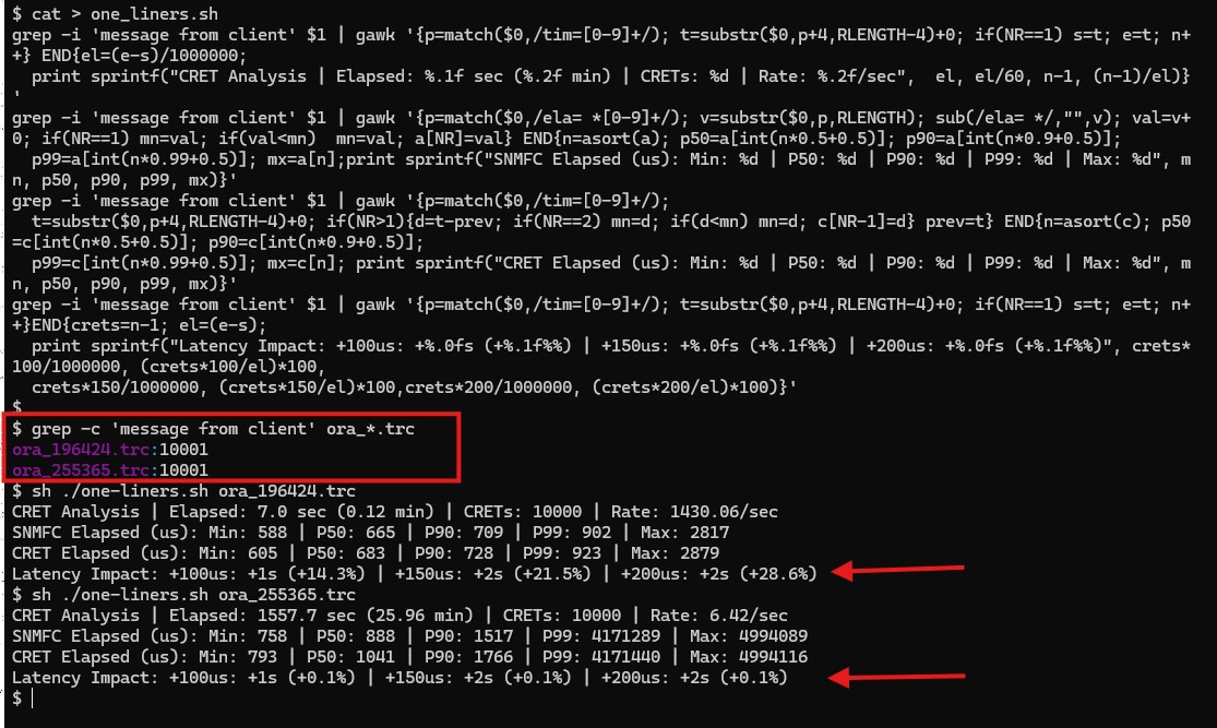
Figure 5: Output of the four CRET one-liner commands for a tight-loop trace and a client-delay trace
Client tight-looping trace (ora_196424.trc)
This trace spans 7.0 seconds, and therefore the 10,000 CRETs averaged 1,430 per second. Dividing 1 second by 1,430 establishes a single-session execution budget of 699µs. The SNMFC P50 of 665µs is the non-database time, which includes both SQLNet RTT and client time. With non-database time consuming 665µs of the 699µs single-session execution budget, there is virtually no room for added SQLNet RTT. One-liner 4 shows that adding, for example, 150µs to SQLNet RTT would add 2 seconds (+21.5%) to the 7 seconds elapsed time. The session processing this SQL statement is not tolerant of meaningful increase in SQLNet RTT latency.
Client-delay trace (ora_255365.trc)
This trace contains 10,000 CRETs produced over 1,557.7 seconds at an average rate of 6.42 CRETs per second, but the session’s execution pattern is bursty and this average is misleading. The SNMFC P99 of 4.17 seconds reveals that multi-second idle periods separate tight bursts of activity, making the per-second average meaningless as a measure of execution intensity. Dividing 1 second by 6.42 establishes a single-session execution budget of ~156ms per CRET. The SNMFC P50 of 888µs (0.888ms) is the non-database time, which includes both SQLNet RTT and client time. With non-database time consuming less than 1ms of a 156ms single-session execution budget, added SQLNet RTT is irrelevant. One-liner 4 shows that adding, for example, 200µs of SQL*Net RTT to each of the 10,000 CRET events adds only 2 seconds to a 26-minute trace. That is a 0.1% increase in elapsed time.
CRET analysis: Side-by-side comparison
| Metric | Example A: Tight-Loop (Sensitive) | Example B: Client-Delay (Tolerant) |
| Total CRETs | 10,000 | 10,000 |
| CRET Rate | 1,430.06 / sec | 6.42 / sec |
| SNMFC P50 (non-DB Time) | 665μs | 888μs |
| SNMFC P99 (non-DB Time) | 902μs | 4,171,289μs (4.17 sec) |
| CRET P50 (Round-Trip) | 683μs | 1,041μs |
| CRET P99 (Round-Trip) | 923μs | 4,171,440μs (4.17 sec) |
| Total Elapsed | 7.0 sec (0.12 min) | 1,557.7 sec (25.96 min) |
| +150μs RTT Impact | +2s (+21.5%) | +2s (+0.1%) |
| Assessment | Not tolerant of added SQL*Net RTT latency | Tolerant of added SQL*Net RTT latency |
Putting it all together
The Client Request Elapsed Time (CRET) Method is a three-phase progressive screening process. Phase 1 uses AWR to identify SQL statements with sub-millisecond database processing time and high execution frequency. Phase 2 assesses SQL Execution Session Density (SESD) to determine whether executions are concentrated in one or very few sessions. If executions are spread across many sessions, the SQL statement is ruled out. If concentrated, Phase 3 involves tracing a high-SESD session and running the CRET Analysis Tool against the trace file to quantify the projected runtime impact of varying increases to SQL*Net RTT.
Interpretation guidance
The methodology projects the runtime impact of increased SQL*Net latency. The following provides a starting framework for migration decision-making.
| Projected Impact | Classification | Guidance |
| < 5% | Tolerant | Workload does not require low SQL*Net latency. Suitable for ODB@AWS. |
| 5% – 10% | Borderline | Warrants discussion with the application owner. Characterize the actual ODB@AWS RTT in the target region before deciding. |
| > 10% | Sensitive | Material degradation expected. Requires RTT characterization, mitigation assessment, or architecture review. |
Connectivity and deployment considerations for ODB@AWS candidates
The following steps help you assess workload compatibility and achieve the lowest possible SQL*Net latency on ODB@AWS:
- Screen your workload first using the CRET methodology.
Before making architectural decisions, complete at least Phase 1 (AWR screening) to identify SQL statements that are fast, frequent, and concentrated (high SESD). This analysis determines whether your workload is a strong candidate for ODB@AWS deployment or requires application-layer optimization first.
- Co-locate the application tier and establish direct ODB Peering.
Deploy latency-sensitive application components in the same Availability Zone as your ODB network to eliminate cross-AZ latency overhead. Establish direct ODB Peering between your application VPC and the ODB network. This provides the shortest possible network path to your Exadata databases without routing through AWS Transit Gateway or AWS Cloud WAN. For detailed connectivity patterns, see Implement network connectivity patterns for Oracle Database@AWS.
- Enable ODB@AWS high-performance networking and validate latency.
Enable ODB@AWS high performance networking to achieve **consistent sub-millisecond SQL*Net round-trip latency** between your application tier (EC2, ECS, or EKS) and ODB@AWS databases within the same Availability Zone. This feature uses automatically provisioned EC2 placement groups to place your application instances in close physical proximity to the Exadata infrastructure at no additional cost. For measurement and validation procedures, see the “Measuring Network Latency” section in Getting started with Oracle Database@AWS high performance networking.
Conclusion
In this post, we presented the CRET methodology, a step-by-step approach to determine whether your workload’s SQLNet latency profile is compatible with the ODB@AWS multi-cloud deployment architecture. By analyzing SQL statements that are fast, frequent, and concentrated, you can identify potential sensitivity to SQLNet latency before migrating.
For workloads identified as latency-sensitive through the CRET assessment, consider reducing SQL*Net round trips by using array fetches, bulk processing, or stored procedures before ruling out the ODB@AWS architecture.