AWS Database Blog
Similarweb’s migration from HBase to Amazon DynamoDB
Managing massive data volumes at scale presents significant operational challenges. At Similarweb we faced these challenges with Apache HBase and found a solution in Amazon DynamoDB.
Similarweb is a digital intelligence platform that provides AI-powered insights into website traffic, app usage, and market trends to help businesses benchmark competitors and optimize growth strategies.
We faced growing scalability and operational complexity issues with our existing Apache HBase infrastructure, which prompted us to explore more flexible and efficient alternatives. This post walks you through our journey migrating our data storage from Apache HBase to DynamoDB. We discuss the technical challenges, migration approach, data modeling strategies, cost optimization techniques, and key benefits achieved along the way. By migrating to DynamoDB, we enhanced performance and scalability and reduced maintenance overhead, so our teams can innovate more rather than focus on infrastructure management. We explore the lessons learned, and the impact this migration had on our business operations.
Background
In our web applications, serving large volumes of data to users requires a robust database solution. That solution must store data effectively, retrieve it quickly, and perform operations such as aggregations, grouping, and sorting before it delivers results to the user interface. To achieve this, we employ a dual approach based on the nature of the data and query patterns, designed to keep the web application responsive and interactive.
Our first approach relates to dynamic queries that depend on user input, or involve complex calculations, such as computing data for power sets of site groups. This can result in an extremely large number of combinations and therefore cannot be feasibly pre-calculated. Therefore, we use cloud analytics databases (OLAP systems), such as Firebolt, for these types of queries. We also use Firebolt for complex query patterns including JOINs, GROUP BY, and other SQL-like query operations. These databases excel at on-the-fly processing of large datasets that aren’t suitable for ETL-based pre-aggregation.
Conversely, our second approach, for features with predictable, pre-calculable access patterns, we rely on key-value (KV) stores such as DynamoDB. By pre-computing data through periodic ETL processes, DynamoDB provides fast and straightforward access to aggregated information, which gives users a responsive experience while balancing performance and scalability.
Requirements for retrieving traffic and engagement data
To illustrate how we use pre-calculated data, let’s walk through a classic use case for website traffic and engagement over time that we show on our platform’s UI.
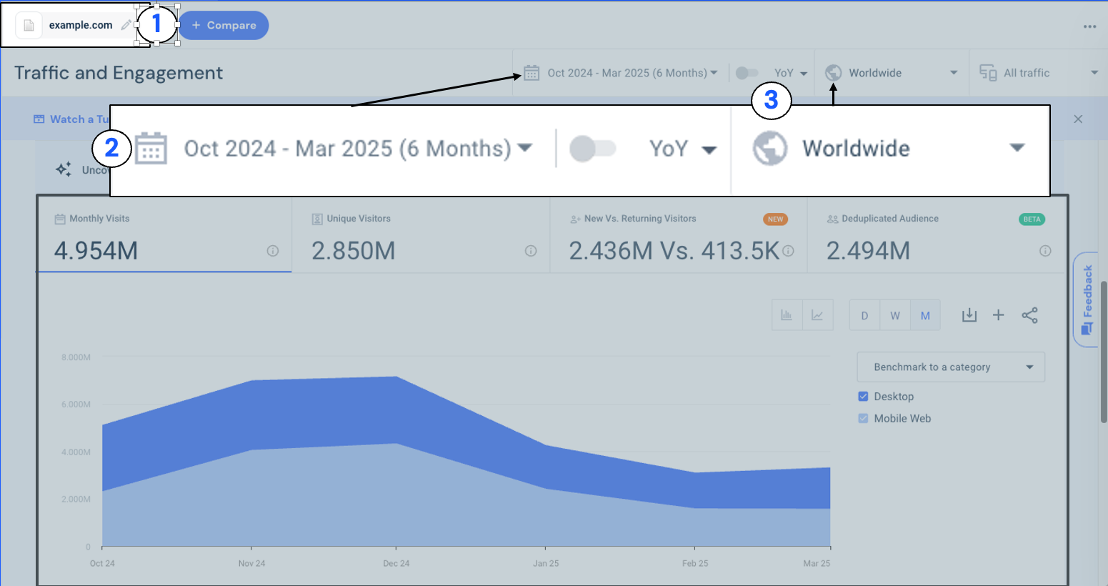
Figure 1: In the Similarweb Traffic and Engagement report, users can select the site to analyze (1), choose a date range (2), and set the geographic scope such as worldwide or a specific country (3). After making these selections, the graph displays key metrics like visits and unique users over the chosen time range.
We store visit statistics for a website, say, example.com, captured with details such as site name, date, country (ISO code), and number of visits.
| Site |
Country (ISO) |
Date | Visits | TimeOnSite | BounceRate | … |
| example.com | 840 | 2026-01-22 | 7 | 15.2 | 7 | |
| example.com | 840 | 2026-01-23 | 11 | 11.7 | 1 | |
| example.com | 840 | 2026-01-24 | 3 | 20.3 | 4 | |
| example.com | 840 | 2026-01-25 | 12 | 13.2 | 5 | |
| example.com | 840 | 2026-01-26 | 9 | 19.1 | 7 |
Our access patterns might involve retrieving all visit data for example.com over a specific date range across all countries or querying the visit data for a specific country, such as the U.S. (840). In this scenario, by pre-computing and storing visit counts for each combination of date, country, and site during the ETL process, we can achieve rapid response times for these common access patterns while minimizing computational overhead at query time.
These pre-computed metrics look simple, but at Similarweb’s scale the underlying write load and query diversity pushed our existing HBase cluster to its limits. In our case, instead of being continuously written, the data is ingested in large batches at scheduled intervals, such as daily, weekly, or monthly, using Spark jobs.
Massive scale and flexible access
At Similarweb, our traffic and engagement datasets are massive, totaling over 255 terabytes (TB). Unlike transactional applications that trickle data in continuously, our analytics pipeline breathes in huge bursts. We ingest approximately 7 billion records per table in tight, scheduled batches that must finish within a couple of hours to keep our data fresh.
However, writing the data is only half the battle. After it’s stored, this data must be instantly available for diverse and complex read patterns. Our users perform more than simple key lookups. They slice and dice data across dimensions to benchmark competitors and analyze trends.
The following figure shows our high-level data flow before the migration.
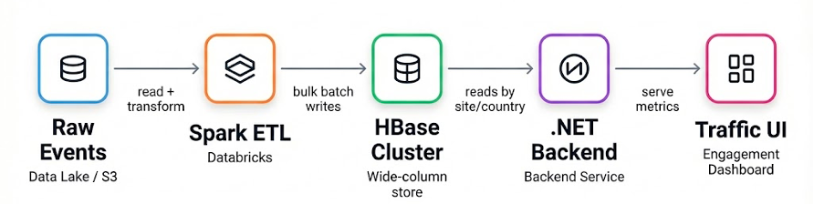
Figure 2 (Before Migration): Raw events land in the data lake, Spark ETL computes daily aggregates, and bulk writes store the results in HBase. The .NET backend reads site and country metrics by key (plus date) and serves them to the Traffic and Engagement UI. All arrows represent data flow.
Beyond simple key-value lookups
We needed a database solution capable of handling massive write spikes while serving single-digit millisecond reads for specific filtering patterns. Specifically, we needed to support these four access patterns for any given site:
- Site-level aggregation: Retrieving all traffic for a site.
- Specific country breakdown: Drilling down into a specific country.
- Time-based trending: Fetching history over a specific window.
- Complex combination: Filtering by both country and date range.
To achieve this, our ideal database had to meet four strict criteria:
- High write throughput: Ingest billions of records in hours.
- Versatile query support: Handle the dimension-based queries listed in the preceding section without scanning full tables.
- Scalability with performance: Maintain high read performance even during peak write times.
- Cost transparency: Provide a predictable pricing model that allows us to estimate costs before execution, rather than being surprised by the bill.
Why HBase hit a wall
HBase served us well for years, but at Similarweb’s scale it gradually shifted from “a database we use” into “a system we operate”. The core limitation was not raw capability. It was the operational risk and instability that appeared after we combined very large batch writes with strict expectations for always-on reads.
1. RegionServer instability became an on-call driver
A recurring source of incidents was HBase RegionServers getting out of sync with the rest of the cluster, or being down. When a RegionServer drifted or misbehaved, it could affect availability and latency for the regions it hosted. Even when recovery was possible, it was unsettling and time-consuming, and it happened often enough to become a real operational burden.
2. Storage and disk upgrades were a nightmare
Managing and upgrading disks in a large HBase footprint was consistently high friction. Disk changes are not isolated events in a distributed system. They ripple through performance, stability, and operational procedures. What should have been routine infrastructure work frequently turned into multi-step maintenance with real risk, especially when we were also trying to protect ingestion windows and read SLAs.
3. The architecture benefits did not match our access patterns
HBase’s wide-column model shines when you read a subset of columns from large rows. In our case, access patterns often required reading the full set of metrics for a key, so we were paying the operational cost of the system without consistently benefiting from its strongest design advantages.
4. High costs because the database was sized for peak
Batch loads in the terabyte range created short, intense write peaks, while the product still needed fast, predictable reads. Keeping an always-on cluster sized for peak meant paying for capacity that we did not actually use most of the day.
These challenges did not show up as a single catastrophic failure. They showed up as accumulated operational toil: more night pages, more time spent on cluster health, and more risk in routine maintenance. That compounding overhead is what pushed us to look for a fully managed alternative.
How DynamoDB addresses these challenges
DynamoDB allowed us to:
- Remove cluster operations from the critical path. With DynamoDB, there are no region servers to provision, no rebalancing, and no manual capacity planning at the infrastructure layer. That directly reduced day-to-day operational work and the number of failure modes tied to database health.
- Scale for batch ingestion without permanent overprovisioning. Our write pattern is predictable: we know how many records we will write and the time window to finish. DynamoDB lets us treat capacity as a dial: we scale provisioned write capacity units (WCUs) up immediately before an ingestion run and scale it back down as soon as it completes. This aligned costs with the batch window instead of forcing us to keep a large cluster running 24/7.
- Keep read performance stable while writes spike. The access patterns behind the UI are mostly key-based lookups and date-range queries. The partitioned architecture of DynamoDB plus Query operations on partition and sort keys let us serve those reads with consistently low latency, even as tables grow very large and ingestion jobs run in parallel.
- Make cost behavior explicit and predictable. Because DynamoDB capacity and request patterns map cleanly to our workload, we can estimate write and read cost from record counts, item sizes, and the expected query shape. That made cost modeling part of the design, instead of an after-the-fact surprise.
- Improve resilience and disaster recovery options. DynamoDB gives managed backups and recovery primitives out of the box. For multi-Region needs, DynamoDB Global Tables can replicate data across Regions so reads can be served locally and recovery does not depend on rebuilding large clusters under pressure.
With this foundation in place, we could focus on the parts that are specific to our workload: how we ingest efficiently at high throughput, and how we model keys to satisfy our access patterns at low cost. The following figure shows our data flow after the migration.
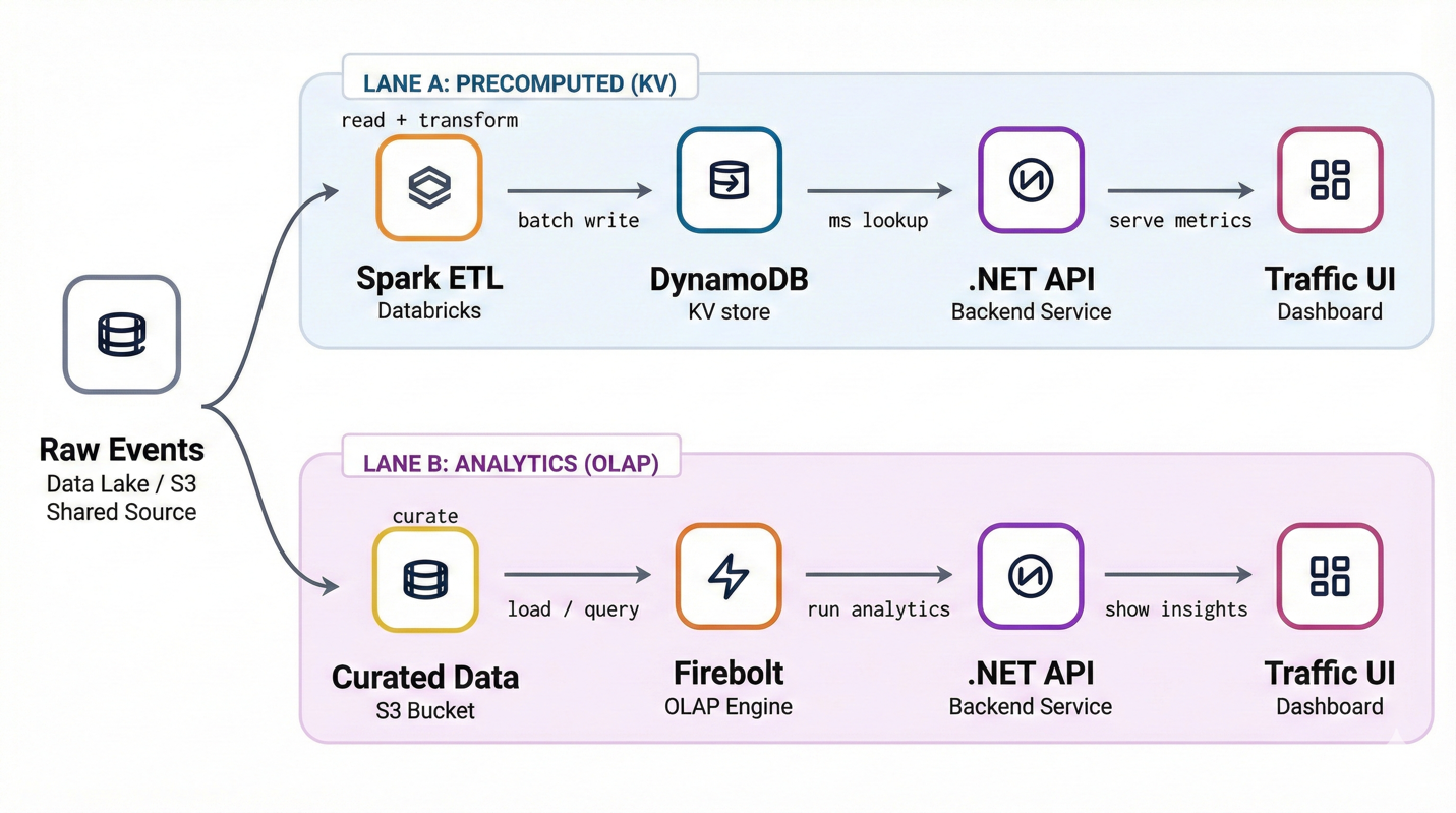
Figure 3 (After Migration): Precomputed traffic and engagement metrics are served through two paths: a key-value lane backed by DynamoDB for predictable, low-latency access, and an analytics lane using Firebolt for dynamic, ad hoc queries. The .NET backend routes requests accordingly. Historically, Lane A used HBase. We replaced it with DynamoDB.
Data modeling
To unlock the full performance and cost benefits of DynamoDB, it was critical to design our data model around our actual query patterns. Our goal was to create efficient access paths that minimize both response times and read/write capacity usage.
Let’s revisit our Traffic and Engagement example, where the core access patterns include retrieving visit data for a site across date ranges, optionally filtered by country.
Naive approach: partition key
An initial approach might be to create a flat, unique partition key like:
| Primary key | Visits | TimeOnSite | BounceRate |
| PK | |||
| example.com_840_2026-01-21 | 4 | 24 | 12.31 |
To retrieve a month’s worth of data, such as visits to example.com in the US (country code 840) during January 2026, we’d generate 31 individual keys and issue a BatchGetItem request:
While this design works, it becomes inefficient and costly at scale. Within a single BatchGetItem request, each item retrieval is counted as a separate read operation, consuming one read capacity unit per item, even when the payload size is small.
Optimal design: composite keys with partition and sort keys
A more scalable model uses composite primary keys with a partition key and a sort key:
- Partition key (PK):
{site}_{country} - Sort key (SK):
{date}
| Primary key | Visits | TimeOnSite | BounceRate | |
| PK | SK | |||
| example.com_840 | 2026-01-21 | 4 | 24 | 12.31 |
With this setup, you can query all records for a site-country pair over a date range using the efficient Query API in DynamoDB:
This reduces the number of API calls and dramatically cuts down on read costs by using range queries on sort keys.
Cost comparison: Query vs BatchGetItem
Consider a use case where you want to retrieve 500 days of data per site-country combination, each entry being ~200 bytes:
Note: RCUs scale with item size in 4 KB chunks. Eventually consistent reads would halve RCUs.
| Approach | Read API | RCU Calculation | Estimated Cost |
| Flat PK | BatchGetItem | 500 items × 1 RCU = 500 RCU | $0.065 |
| Composite PK + SK | Query | 100 KB / 4 KB = 25 RCU | $0.00325 |
Savings: Over 20x cheaper using a composite key design.
Worldwide use case
While our composite key model, PK = {site}_{country}, SK = {date}, efficiently supports common queries filtered by site, country, and date range, it introduces a challenge when we need to query visit data across all countries. For example, retrieving all visits to example.com worldwide, either for all time or within a specific date range:
In our existing schema, the country code is embedded in the partition key, which is essential for evenly distributing write and read load across partitions. However, this also means that you must know the country in order to query the data, something we don’t want for global aggregation use cases.
A straightforward but inefficient solution is to fan out Query API calls across every country-specific partition:
While functionally correct, this approach has several drawbacks:
- High cost: Over 200 Query requests per site/date query.
- Increased latency: Querying and aggregating results across 200 queries can significantly increase response time.
- No BatchQueryItem: Unlike BatchGetItem, there’s no native way to batch multiple Query requests into a single API call.
- Operational overhead: Managing 200+ parallel queries can put load on the application and increase risk of throttling.
To support efficient global queries without incurring the cost and complexity of fan-out, we introduced a special synthetic country code (for example, 999) during the ETL process. In practice, we precompute and store aggregated worldwide metrics as part of the ETL pipeline and write them to a dedicated “global” partition. This is done by using a designated partition key for worldwide data, where PK = {site}_999.
| Primary key | Visits | TimeOnSite | BounceRate | |
| PK | SK | |||
| example.com_840 | 2026-01-21 | 4 | 24 | 12.31 |
| example.com_999 | 2026-01-23 | 33 | 17 | 16.5 |
This enables querying worldwide data with a single Query request:
This way we don’t have any performance overhead while reading, while also incurring less cost because we use one Query request instead of multiple.
Of course, the “999” approach is not without cost. It adds extra ETL complexity because we now need to compute an additional worldwide rollup per site and date, and it also increases storage because we persist an extra item alongside every site-country record. Still, when we look at the system end to end, it’s a clear win. We shift work from read time to write time, eliminate the need for 200+ fan-out queries, reduce application-side orchestration, and get consistently faster worldwide reads. In practice, the added ETL and storage cost is outweighed by the savings in query cost and latency, so the overall solution ends up cheaper and faster.
In the next section, we explore how we further use DynamoDB features to save time and costs during initial data migration and monthly data ingestion.
Writing to DynamoDB
Batch ingestion is the heartbeat of our analytics pipeline. Instead of a continuous stream, we rely on scheduled Apache Airflow Directed Acyclic Graphs (DAGs) that trigger ETL Spark jobs on Databricks at daily, weekly, or monthly cadences, each tuned to the freshness requirements of its downstream feature. Every run pushes billions of items, often several terabytes, to DynamoDB in a short time window so the tables are ready for read traffic as soon as possible.
DynamoDB offers two distinct capacity modes to fit different workload patterns. The on-demand mode is a serverless, pay‑per‑request model that automatically scales to meet traffic demands, with no capacity planning required and you pay only for what you use. In contrast, the provisioned mode requires you to specify the read and write throughput that you want ahead of time, and billing is based on this provisioned capacity whether fully used or not. In our case, because we already know the total number of records to write and the time window for ingestion, we can precisely calculate and set the write capacity units needed. This makes provisioned mode significantly more cost‑effective than on‑demand for our scheduled batch loads.
End-to-end batch workflow
- Airflow schedules the load
- DAG parameters include table name and the date ranges for reading from the source.
- Jobs are staggered to avoid overlapping peaks.
- Databricks Spark runs the ETL
- Spark partitions align with the DynamoDB partition key to maximize parallelism.
- We use the DynamoDB Connector for Apache Spark, which batches writes and handles retry logic with exponential back-off.
- Capacity is scaled up just-in-time
- Before the first write to the target DynamoDB table, our infrastructure script calls UpdateTable to raise the table’s provisioned write capacity, or write capacity units (WCU), to the calculated peak. The script sets this level automatically based on the target duration and the record count.
- Data is written in parallel
- We use the DynamoDB Connector for Apache Spark to write data at a throughput closely aligned with our provisioned capacity. Typically, we target about 1.1 times the provisioned write capacity, accepting a controlled level of throttling to achieve optimal utilization without underutilizing our resources.
- Capacity is scaled back down automatically
- As soon as the ETL finishes writing all records, we schedule a follow-up task that calls UpdateTable again to lower the provisioned capacity write level.
Python pseudocode of calculating and scaling up DynamoDB table’s provisioned capacity
Using Import Table from Amazon Simple Storage Service (Amazon S3)
To further reduce the time and cost of writes to DynamoDB, we used the DynamoDB Import from S3 feature to import data directly from Amazon Simple Storage Service (Amazon S3) when migrating from HBase and for some periodic writes. This eliminates the need for per-record writes and avoids consuming write capacity units during ingestion.
Benefits
- Up to 90% cost reduction for bulk ingestion.
- No Databricks compute usage required for ETL ingestion.
- Simplified operations with retry logic hidden and operational overhead removed by the native import.
- Faster ingestion compared to our conventional Spark jobs.
Since the Import Table feature charges based on the total volume of data ingested rather than per-item write operations, it offers significant cost savings, especially when migrating large tables with small items, like in our case.
Import from S3 workflow
- As part of the pre-ETL automation, data is read from the specified S3 path and converted into the DYNAMODB_JSON format supported by the Import from S3 feature.
- We invoke the ImportTable API with the S3 path of the formatted data and table definition.
- A monitoring task tracks the progress until the import completes.
When to store data in separate tables by period
DynamoDB Import from S3 feature is a game changer for large backfills, but it comes with an important constraint: it can only import into a new table. That limitation becomes an opportunity if your dataset is naturally time-partitioned and primarily accessed by recent periods.
For monthly datasets, we adopted a deliberate design: create one table per month, import that month’s data using Import from S3, and manage the lifecycle of those tables as the data ages.
Why this works well for monthly data
This approach fits monthly workloads especially well because:
- Bulk loads are discrete: each month’s dataset is typically produced as a complete batch, making it a clean unit for import.
- Operational simplicity at query time: applications can route queries to the relevant period table(s) instead of mixing cold and hot data in one large table.
- Retention becomes trivial: instead of deleting old items, you can drop entire tables when they expire.
- Cost optimization is easier: older monthly tables can move to Standard-IA table class as they age, reducing storage cost without changing application logic.
A practical naming convention makes this easy to automate, for example: {table_name}_2026-01.
How we run it end to end
- For each month, we generate the dataset, convert it to DynamoDB JSON, one of the supported import formats, and run ImportTable into a new monthly table.
- After import, we apply a retention policy that removes tables once they are no longer needed.
- We transition aging monthly tables to Table Class Standard-IA to save on storage costs.
- When a requested date range spans multiple months, the API fans out queries across the relevant monthly tables and merges results.
When not to use period-based tables
This pattern is powerful, but it is not universal.
For daily datasets, creating a table per day would explode the number of tables and introduce unnecessary operational overhead. In those cases, it’s better to keep a single long-lived table and continue with the standard ingestion path: Spark writes + provisioned capacity scaling.
Rule of thumb
- Prefer separate tables by period when the period is coarse (monthly or larger), the data is loaded in bulk, and retention can be enforced at the table level.
- Prefer a single table when periods are too fine-grained (daily), or when you need continuous incremental writes into the same physical table.
Conclusion
In this post, we showed how Similarweb migrated from Apache HBase to DynamoDB. This transition was driven by the need to simplify operations, scale efficiently, and reduce infrastructure overhead while continuing to deliver fast, reliable insights at scale.
Our legacy HBase setup, while powerful, struggled to meet the growing demands of our batch ingestion workflows and dynamic query requirements. Challenges like stability, operational maintenance, and scaling limitations prompted us to seek a more modern, serverless alternative.
By adopting DynamoDB, we achieved:
- High-performance batch ingestion using ETL jobs with intelligent write provisioning.
- Flexible and cost-efficient data modeling that supports diverse query patterns at scale.
- Reduced operational burden through the fully managed and serverless DynamoDB architecture.
- Low operational burden and fast historical data migration by importing directly from Amazon S3.
- Improved system reliability and scalability without the need for manual cluster management.
This migration enhanced the performance and stability of our data infrastructure and freed up our engineering teams to focus on building features and driving innovation. DynamoDB has proven to be a resilient and cost-effective foundation for our analytics pipeline, supporting Similarweb’s mission to deliver timely, actionable digital insights to our customers.