Networking & Content Delivery
Measuring network latency to AWS Region before deployment
The problem: choosing the right Region when geography gets complicated
Considering network latency before deployment, many teams follow a basic rule: pick the AWS Region closest to their users. But real-world constraints can make this decision more complex than it appears. It may require actual latency measurement rather than geographic assumptions. This post provides a step-by-step procedure for measuring network latency to AWS Regions before deployment. We’ll also explore how to interpret basic latency test results and understand the routing factors that influence latency measurements. This pre-deployment basic latency data gathering approach can save approximately 1-2 hours, compared to deploying infrastructure directly to the target region to test against.
Note: Existing AWS blog posts cover latency measurement for deployed infrastructure. These posts show how to use tools like Amazon CloudWatch Internet Monitor and AWS Network Manager against live endpoints. This post addresses different challenges. How to measure real network latency to candidate AWS Regions before deploying resources utilizing free, publicly available tools.
Consider this scenario: You’re building an Amazon Elastic Kubernetes Service (EKS) environment to serve downstream users in Palm Springs and Palo Alto, California. The natural choice is us-west-1 (N. California). However, us-west-1 has constraints that you might encounter:
- New accounts restrict you to only two Availability Zones, which limits your high-availability architecture options.
- Certain instance types might have limited availability compared to larger Regions.
- Some AWS services don’t launch simultaneously across every Region.
Consider us-west-2 (Oregon) as an alternative. It offers more Availability Zones, broader service availability, and better capacity, but it’s farther away. You need to determine whether the additional network latency is acceptable for your application’s requirements.
The challenge is measuring latency before deploying resources.
The solution: looking glass sites and Amazon EC2 reachability endpoints
You can overcome this challenge without deploying any infrastructure by using two publicly available tools in a 4-step process that takes approximately 15-30 minutes to complete. Deploying test infrastructure typically involves 1.5-2.5 hours for resource provisioning and configuration, plus additional time for cleanup. You can get preliminary latency data before spending hours on infrastructure deployment. This approach provides preliminary measures of latency in under an hour at zero cost. It provides you with data to make informed Region decisions before deployment.
Figure 1 shows the pre-deployment latency validation workflow.
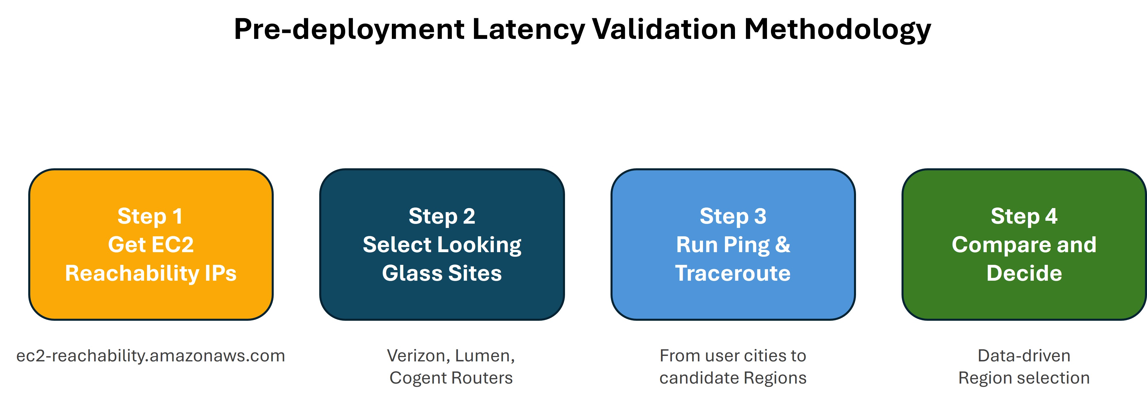
Figure 1: Pre-deployment latency validation workflow
Prerequisites
A knowledge of basic networking concepts, and access to a web browser and an internet connection.
Step 1: Identify pingable targets in your candidate Regions
You can find a set of reachable endpoints for network testing at ec2-reachability.amazonaws.com. This page provides IP addresses for Amazon Elastic Compute Cloud (Amazon EC2) instances in supported AWS Region that respond to ICMP ping and TCP reachability checks.
To identify your target endpoints
- Navigate to http://ec2-reachability.amazonaws.com/ in a browser.
- Make note of IP addresses for each Region you’re evaluating.
- Record the addresses for your candidate Regions.
These endpoints give you a consistent, AWS-maintained target in each Region. You don’t need to deploy an EC2 instance to test against. They support both ICMP and TCP-based reachability checks. AWS might apply rate-limiting, so space your tests accordingly and avoid automated high-frequency polling.
Step 2: Use looking glass sites to test from specific locations
Major network carriers provide looking glass tools for running diagnostic commands from their routers in various cities. You don’t need to physically be in Palm Springs or Palo Alto to test latency from those locations.
You can use looking glass tools to simulate network tests from your end users’ geographic locations without having infrastructure there.
Important note: Looking glass tool availability varies by carrier. Providers might discontinue, restrict, or change access over time. We validated the following looking glass URLs before publication. You can also search for additional looking glass sites or ask your ISP if they offer one.
Public looking glass tools:
| Provider | URL | Notable locations |
| Verizon | https://www.verizon.com/business/why-verizon/looking-glass/ | Palo Alto, Los Angeles, Dallas, NYC |
| Lumen (CenturyLink) | https://lookingglass.centurylink.com/ | Broad US and international coverage |
| Cogent | https://www.cogentco.com/en/looking-glass | Major metro areas globally |
Step 3: Run the tests
To run a looking glass test
- Open a looking glass site.
- Choose a router location close to your users or data center.
- Choose ping or traceroute as the test type.
- Enter the IP address from the EC2 reachability page for your target Region.
- Run the test and note the round-trip time (RTT).
- Repeat for each candidate Region and user location.
Interpretation guidance: A single ping test is a point-in-time measurement. Run tests at multiple times of day (morning, afternoon, evening) to understand variability. If you encounter RTT variance greater than 30% at different times, network congestion or routing changes are likely factors. Test from multiple carriers to isolate the cause.
Step 4: Compare results and make a decision
Ping Testing
For the example scenario, you might see ping results like:
- Palo Alto, CA to us-west-1 (N. California): ~5-10 ms
- Palo Alto, CA to us-west-2 (Oregon): ~15-25 ms
Ping RTT ranges and application viability
| Latency | Workloads |
| 5-15ms | Excellent for latency-sensitive applications, such as real-time voice and video. |
| 15-50ms | Good for most web applications and APIs. May impact real-time applications depending on requirements. Acceptable for most database operations. |
| 50-100ms | Noticeable delay for interactive applications. Still acceptable for batch processing and background tasks. Evaluate user experience impact for web applications. |
| 100ms+ | Significant latency that will impact user experience. Only suitable for non-interactive workloads. May indicate routing issues or very long geographic distance. |
Note: ICMP round-trip latency is not a measure of application latency. Application latency includes additional overhead from TCP, TLS, DNS, and the application layer. But this approach should provide sufficient data to inform your deployment decision for that Region. Then, you can move to the next step, performing a true end-to-end application test from the target Region.
If you were to see RTT values like 45ms to us-west-2, several factors should be evaluated:
Geographic distance: Physical distance between test location and AWS Region
Internet service provider routing: Your ISP’s network path to AWS
Peering relationships: How your ISP connects to AWS’s network
Network congestion: Traffic levels on the path at test time
To investigate these factors further, run a traceroute test from the same looking glass location to see the network path and identify where latency accumulates. Ping provides a single round-trip time number. Traceroute illustrates where the path introduces latency, which helps you understand whether latency comes from geographic distance or from inefficient routing.
Interpreting traceroute results
A traceroute from the Verizon Palo Alto router to a us-west-2 target produces output similar to the following example:
Figure 2 illustrates where latency is introduced at each hop along the traceroute path.
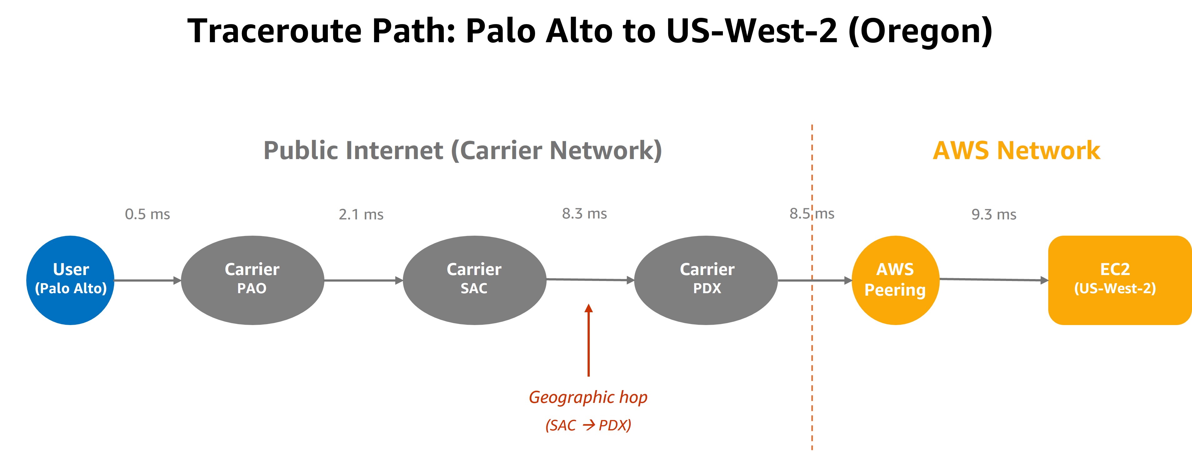
Figure 2: Traceroute path showing where latency is introduced at each hop
What to look for in your traceroute:
| Pattern | What it means |
| Large jump between two hops (for example, 2 ms to 8 ms) | Geographic distance between those routers. City codes in host names indicate location (PAO = Palo Alto, PDX = Portland, ORD = Chicago). |
| Consistently low increments | Good peering and direct routing. Traffic takes a logical geographic path. |
| Unexpected city codes mid-path | The network backhauls traffic through intermediate sites. For example, Palo Alto traffic routes through Dallas before reaching Oregon, this represents inefficient routing. |
| * * * (timeouts) mid-path | The router at that hop doesn’t respond to traceroute probes. Many core routers deprioritize ICMP; this isn’t necessarily a problem. |
| High latency only at the final hop | Possible indication of load on the target instance rather than a network path issue. |
Understanding BGP path influence
The route your traffic takes to AWS depends on BGP (Border Gateway Protocol) peering arrangements between your ISP or carrier and AWS. Testing from multiple looking glass providers matters because each carrier has different peering.
Direct peering: Your carrier peers directly with AWS at a local exchange point (for example, the Equinix facility in San Jose). Traffic takes the shortest path.
Transit routing: Your carrier doesn’t peer directly with AWS in your metro area. Traffic might transit through a third-party backbone and enter AWS at a more distant point of presence.
AWS edge locations vs. Region entry points: In most cases, traffic enters AWS’s network at the nearest peering point, then traverses AWS’s private backbone to reach the target Region.
Figure 3 illustrates the difference between direct peering and transit routing.
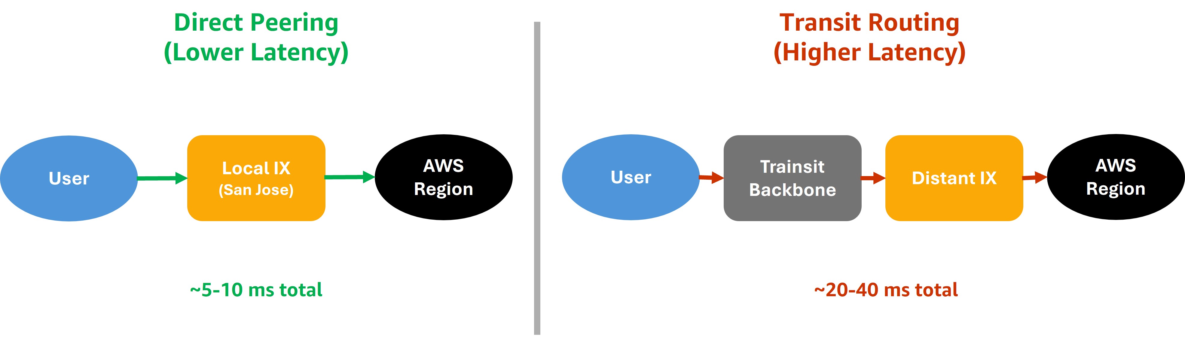
Figure 3: Direct peering vs. transit routing and the impact on latency
Practical tip: In the traceroute output, look for the hop where the host name changes to an Amazon-owned address. Examples include 52.93.x.x, amazon.com in the reverse DNS, or aws in the host name. The city where this handoff occurs tells you where your traffic enters AWS’s network.
Multiple carriers, different paths
Verizon, Lumen, Cogent, and other ISP’s each have different peering arrangements with AWS:
- One carrier might peer with AWS directly in a local metro area.
- Another might hand off traffic at a distant exchange point.
- A third might have congested peering links that add jitter (a variation in latency).
- Some might not peer with AWS directly, and must traverse an intermediary network.
Decision point: If you see significantly different latency between carriers from the same city, investigate further. The difference is almost certainly because of peering topology, not geography. This finding can inform ISP selection or justify a dedicated connection through AWS Direct Connect.
When this approach is most useful
Use this technique when:
- You’re evaluating a new Region and want to validate latency assumptions before committing to infrastructure.
- You have users in multiple cities and you want to find the Region that best serves each of them.
- You’re considering a Region migration (for example, from us-west-1 to us-west-2) and need to quantify the latency impact.
- You want to validate connectivity to a Region from a specific carrier because ISP peering matters for your use case.
- A Region has constraints (capacity, AZ count, service availability) and you need data to justify choosing a farther Region.
Important considerations
Looking glass limitations
Looking glass tests show latency from the carrier’s router in that city, not from your exact data center or office. The last-mile hop adds some latency, but it’s usually a small delta. Results vary by time of day and network conditions. Run tests at multiple times for a realistic picture.
Carrier peering limitations
Different carriers have different peering arrangements with AWS. Test from multiple providers for a more complete view. Carrier looking glass tool availability is not guaranteed. Always verify availability before relying on a specific provider.
Amazon EC2 reachability endpoint considerations
The endpoints respond to ICMP ping and TCP-based reachability checks. Verify current protocol support on the reachability page before testing. AWS might apply rate-limiting. Space tests appropriately and don’t use automated high-frequency polling. These are shared public endpoints intended for basic connectivity validation, not sustained performance benchmarking.
Beyond ping: other Region selection factors
Latency is one factor in Region selection. Also consider:
- Available services: Does the Region support the services your architecture requires?
- Availability Zones: Do you require three or more AZs for your high-availability design?
- Capacity: Are the instance types you require readily available?
- Compliance: Do data residency requirements dictate a specific Region?
- Cost: Pricing can vary slightly between Regions.
For ongoing monitoring after deployment
The looking glass approach is best for the pre-deployment decision phase. After you’ve deployed, AWS provides tools for ongoing latency monitoring:
You can monitor internet performance between your users and AWS, quickly detect and diagnose issues, using Amazon CloudWatch Internet Monitor.
You can visualize your entire global network, including latency and packet loss metrics between your sites and AWS Regions, from a single console using AWS Network Manager.
For use cases where no single Region provides ideal latency for identified user locations, Amazon Route 53 latency-based routing directs users to the lowest-latency endpoint automatically.
Summary
This post shows how you can measure network latency to AWS Regions without deploying infrastructure. By combining AWS’s published EC2 reachability endpoints with carrier-provided looking glass tools, you can gather real latency data from the cities that matter to your application.
This approach removes guesswork from Region selection and helps you confirm your chosen Region meets your performance requirements, even when the closest geographic option has constraints that push you elsewhere.
Have questions about measuring latency to AWS Regions, or want to share your own approach? Share your questions or your approach in the comments below.
Key takeaways:
- Amazon EC2 reachability endpoints provide free, AWS-maintained ping targets in each supported Region.
- You can use carrier looking glass tools to test from specific geographic locations where you don’t have existing infrastructure.
- Trace route analysis reveals whether latency is geographic (inherent) or routing-related (addressable).
- Testing from multiple carriers exposes peering differences that affect real-world performance.
- Preliminary testing can be completed in under an hour at zero cost.
Clean up resources
This approach uses only free, publicly available tools and doesn’t deploy any AWS infrastructure. No resources require cleanup.
Additional resources
For more information on network performance measurement and Region selection:
- Network latency concepts and best practices for a resilient architecture (AWS Networking and Content Delivery Blog)
- What to consider when selecting a Region for your workloads (AWS Architecture Blog)
- Amazon EC2 Reachability Test
- AWS Global Infrastructure
About the author

Chris Mahanna
Chris is a Sr. Technical Account Manager at AWS supporting Media and Entertainment customers. He helps organizations design resilient network architectures and make data-driven infrastructure decisions. Outside of work, Chris enjoys spending time with his wife, his children, and their golden retriever, Sadie.