Thermodynamic sampling of disordered materials with an analog Hamiltonian Rydberg simulator

This post was contributed by Mao Lin, Bruno Camino, John Buckeridge and Scott M. Woodley

Many advanced materials — from battery electrodes to semiconductor alloys — owe their useful properties to atomic-scale disorder. But predicting how atoms arrange themselves at a given temperature is hard: the number of possible configurations explodes combinatorially and sampling them according to their thermodynamic weights can overwhelm classical computation.

In this post, we report results from our recent publication demonstrating how the QuEra Aquila device, available through Amazon Braket, can serve as a thermodynamic sampler for realistic material models [1]. Using quantum annealing, we map an energy model derived from classical density functional theory (DFT) onto the neutral atom quantum hardware and sample low-energy configurations of nitrogen-doped graphene. We validate the approach on a 28-site system via exhaustive enumeration, benchmark it on a 78-site system against classical Monte Carlo sampling and demonstrate temperature tuning through programmable atom spacing.

Mapping disordered graphene to Rydberg atoms

To determine the equilibrium dopant concentration as a function of temperature and chemical potential for nitrogen doped graphene, we consider graphene nanoflakes (a single layer of carbon atoms arranged in a honeycomb lattice) where each lattice site can be occupied by either a carbon or a nitrogen atom. Pure graphene, Figure 1(a), is taken as a reference state, and the energy of doped configurations is measured relative to this reference. Importantly, dopants do not contribute independently, and they interact with one another such that the energy depends not only on how many dopants are present but also on their relative arrangement on the lattice. In particular, the interaction strength decays with dopant separation so that the farther apart two dopants are, the weaker their mutual interaction. See Figure 1(b) for an illustration of the mapping and the interaction effects of the dopants.

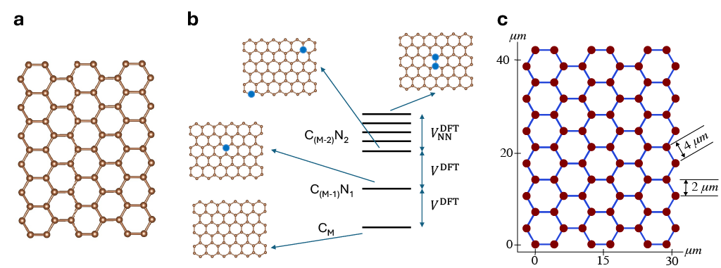
Figure 1 – Illustration of mapping a doped graphene to Rydberg atoms. (a) A pristine graphene with 78 sites, each site can be occupied by either a carbon (gold) or a nitrogen atom (blue). (b) The energy levels of the doped graphene systems measured with respect to the pristine graphene (CM). Doping the graphene with a nitrogen atom (C(M-1)N1) increases the energy of the system by VDFT, the on-site energy of the dopant, whereas the energy of systems with two dopants (C(M-2)N2) depend also on the distance of the dopants. When the two dopants are next to each other, its energy relative to the pristine graphene is 2VDFT+VNNDFT where VNNDFT is the nearest neighbor interaction energy of the dopants. (c) The largest layout for the Rydberg atom simulator used this work which contains 78 sites. A valid layout must comply with the constraints that the nearest neighbor spacing is not less than RNNmin=4 μm and the y-coordinate difference between any two sites is not less than 2 μm.

We encoded the energy levels of a doped graphene using Rydberg atoms. In this setting, each atom acts as an effective two-level system with a ground state |g⟩ and a Rydberg excited state |r⟩, driven by a global laser field and coupled through distance-dependent Rydberg interactions. We chose to map carbon and nitrogen atoms to the ground and Rydberg states, respectively. A commonly used model for the resulting analog dynamics is the time-dependent Hamiltonian

Here n_i is the Rydberg occupation operator, Ω(t) is the global Rabi frequency controlling coherent transitions between the ground and Rydberg states, Δ(t) is the global detuning that biases Rydberg excitation, and C₆ is a constant that determines the van der Waals interaction between atoms i and j set by the programmable inter-atom spacing R_i,j. The cost function H_cost is a time-dependent function that depends on the global detuning, atom arrangement and the distribution of the Rydberg occupations.

At the end of the quantum annealing evolution, we want the Rydberg Hamiltonian to reproduce the same relative energy ordering and thermodynamic weights as the classical DFT formation-energy landscape of the doped graphene. To accomplish this we construct a training set of N_train doped graphene configurations represented as binary occupation vectors (carbon = 0 and nitrogen = 1), calculate the corresponding DFT formation energies, then solve the linear regression:

The resulting parameters, V^DFT and R_i,j^DFT, are used to parameterize the final time H_cost and the subsequent quantum annealing procedure on the Rydberg hardware.

The overall energy scale of the DFT-derived model is not commensurate with the scale accessible in the Rydberg device. Specifically, after solving the linear regression, the resulting parameters are orders of magnitude larger than what the device can realize given its bounded detuning range and the maximum van der Waals interaction set by the minimum allowed spacing R_NN^min between the nearest-neighbor atoms. In other words, the nearest-neighbor spacing obtained by DFT, R_NN^DFT, is much smaller than R_NN^min.

We address this mismatch of energy scales by defining a single uniform rescaling factor α_V=(R_NN^min/R_NN^DFT)⁶ that compresses the entire DFT energy model into the device’s dynamic range. The largest target coupling is realized at R_NN^min while preserving relative energy differences and thus the Boltzmann weights up to a temperature rescaling. The device therefore samples the original graphene thermodynamics at an effective temperature T’=α_VT_eff where T_eff is a parameter to be calibrated. Moreover, because the nearest-neighbor spacing R_NN is a programmable hardware choice (subject to R_NN ≥ R_NN^min), adjusting R_NN provides a means to tune the effective temperature of the sampling, and hence study the temperature dependence of the dopant concentration.

Imperfect quantum annealer as a thermal sampler

In this work, we use an analog Hamiltonian Rydberg simulator as a quantum-annealer, which is often described as a ground-state finder. But this is the ideal limit of a perfectly isolated, zero-temperature, infinitely slow evolution. In practice, an analog Rydberg simulator runs for finite time and is weakly coupled to the environment, so its output is better viewed as a heuristic sampler that preferentially returns low-energy configurations rather than a deterministic optimizer. This is exactly what thermodynamic sampling requires: at temperature T, equilibrium assigns each configuration z, say a dopant pattern, probability P(z, T) ∝ exp(-E(z)/k_BT), so the goal is not to always return the configuration that minimizes E(z), but to return low-energy configurations with higher frequency according to their Boltzmann weight. Empirically, many annealing devices produce output distributions that are often reasonably approximated by P(z, T_eff) for some effective temperature T_eff that can be calibrated [3-6]. In this perspective, the same non-idealities that limit guaranteed ground-state preparation — finite temperature, control noise, and incomplete adiabaticity — become a feature: they provide the mixing needed to sample an ensemble. For disordered materials, where thermodynamic observables are dominated by a relatively small set of low-energy configurations, a device that repeatedly produces Boltzmann-biased samples can be directly useful even without perfect equilibration over the entire configuration space.

Results

We report three experiments: effective-temperature calibration on a 28-site system, a 78-site benchmark against unbiased Monte Carlo, and temperature tuning through the programmable nearest-neighbor spacing.

Calibrating the effective temperature. We first validate the mapping and calibrate the sampler’s effective temperature on a small instance where exhaustive search is possible. Using a 28-site graphene nanoflake mapped to a Rydberg-atom array with nearest-neighbor spacing fixed to the hardware minimum, we run the QPU at 10 final detuning values, which effectively vary the chemical potential of the system, and measure the resulting average nitrogen concentration. We then compute the exact equilibrium prediction by exhaustively enumerating all 2²⁸ configurations and evaluating Boltzmann probabilities over a range of temperatures (1-60 μK). By minimizing the root mean squared error between the QPU curve and the exhaustive-search curve, we identify an effective sampling temperature of T_eff=41μK. The result of this benchmark is shown in Figure 2(a).

Benchmarking against Monte Carlo. We then move to two larger-scale experiments that illustrate the thermodynamic controls available on this Rydberg-atom simulator. First, on a 78-site nanoflake (shown in Figure 1(a)), where full enumeration is infeasible, we tune the chemical potential Δμ by sweeping the global detuning and comparing against unbiased Monte Carlo (UMC) that samples random configurations uniformly. At the calibrated T_eff=41μK and R_NN=4μm, Figure 2(b) shows that the QPU reproduces the expected monotonic dependence of the average dopant concentration on Δμ. We observe that, in the intermediate regime (-Δ_g<0 where Δ_g is the global detuning), the Monte Carlo predictions approach the QPU results as the Monte Carlo sample size is increased, highlighting that accurate UMC estimation can require very large numbers of samples. For each QPU data point, we executed 1000 shots for the annealing protocol and retained only runs corresponding to fully occupied initial configurations when computing the averages (ranging from 40.6% to 81.4% of the shots). This result is noteworthy: the quantum processor produces accurate thermodynamic estimates from 1000 shots, while UMC requires substantially more samples to converge to the same result in the correlated regime.

Tuning temperature via atom spacing. We demonstrate a direct temperature-control knob available in the Rydberg platform through the programmable nearest-neighbor spacing R_NN. Because the Rydberg interaction strength depends strongly on distance, changing R_NN changes the effective energy scale of the implemented Hamiltonian and, under our mapping, corresponds to sampling the graphene model at different effective temperatures. Figure 2(c) shows the resulting dopant concentration for three spacings (R_NN=4.0, 4.5, 5.0μm), which correspond to three effective temperatures (as indicated in the legend). We observe that as the temperature is lowered (equivalently R_NN is decreased), the curve systematically shifts towards a sharper distribution as expected, illustrating how geometry control can be used to probe the temperature dependence of dopant thermodynamics on

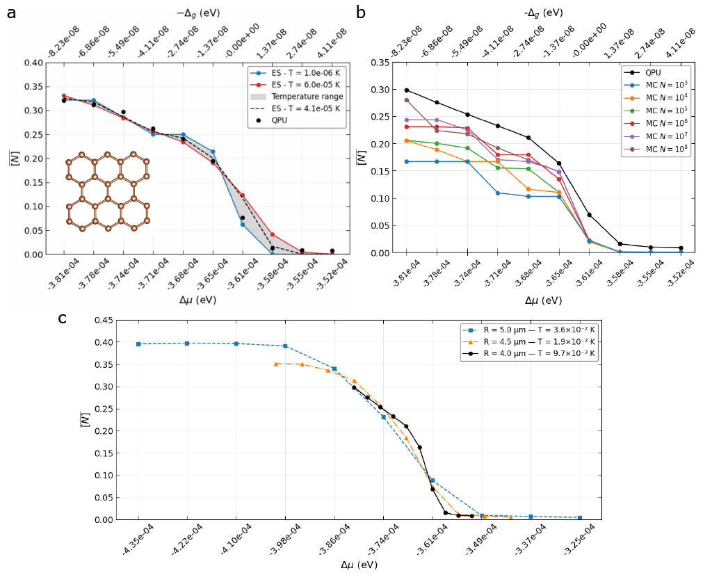
Figure 2 – Result of the thermodynamic sampling. (a) Effective temperature calibration with a 28-site nanoflake as shown in the inset. The horizontal axis represents the chemical potential, or equivalently the global detuning, and the y-axis is the average concentration. Comparing the QPU data to the exhaustive search result yields Teff=41μK. (b) The average concentration as a function of chemical potential. We compare the QPU data with UMC of different sample sizes. (c) The average concentration as a function of temperature and chemical potential. As we lower the temperature, the curve is shifted towards a sharper distribution as expected.

Conclusion

This work presents a proof-of-concept demonstration using a Rydberg-atom quantum processor as a thermodynamic sampler for realistic, DFT-informed models of disordered materials, enabling direct estimates of finite-temperature equilibrium properties without exhaustive enumeration. For a detailed technical discussion, see our full paper [1]. To get started with Amazon Braket, refer to our example notebooks. Researchers from accredited institutions can apply for the AWS Cloud Credit for Research program by submitting a research proposal here.

References

[1] B. Camino, et al. (2025). Thermodynamic sampling of materials using neutral-atom quantum computers. npj Quantum Information (2026)

[2] B. Camino, et al. (2025). Exploring the thermodynamics of disordered materials with quantum computing. Science Advances 11(23), 7156 (2025).

[3] J. Marshall, et al. (2017). Thermalization, freeze-out and noise: deciphering experimental quantum annealers. Physical Review Applied 8, 064025 (2017).

[4] M. Benedetti, et al. (2016). Estimation of effective temperatures in quantum annealers for sampling applications: A case study with possible applications in deep learning. Physical Review A 94, 022308 (2016).

[5] J. Raymond, et al. (2017). Global warming: Temperature estimation in annealers. Frontiers in ICT 3 , 23 (2016).

[6] J. Nelson, et al. (2022). High-Quality Thermal Gibbs Sampling with Quantum Annealing Hardware. Physical Review Applied 17, 044046 (2022).