AWS Storage Blog
Accelerate inference with KV cache tiering on AWS
When running large language model (LLM) inference at scale on AWS, the GPU might not be the only thing that limits you. The GPU generates tokens fast, but what then contributes to performance is everything around it: memory, storage, and the network path that connects them. That’s the difference between a demo and production. Training is predictable; you know how many GPUs, how long, and how much data. Inference is unpredictable, latency-sensitive, and scales with every concurrent user you add. Because inference is your daily production workload, its economics live beyond the GPU; they live in the memory hierarchy that feeds it.
At the center of this challenge sits the key-value (KV) cache. As context windows grow to millions of tokens and agentic workflows maintain persistent sessions, KV cache has become the binding constraint on accelerator utilization and cost per token. For large-scale models, reading KV cache back from shared storage is far less costly than recomputing it, at any context length. The question isn’t whether to store KV, it’s where to put it and how fast you can move it. This post presents a four-tier storage framework for sizing, placing, and moving KV cache across your inference fleet, so you can maximize token throughput without overprovisioning memory.
This framework applies equally to AWS Trainium instances (Trn2, Trn3 UltraServer) and NVIDIA GPU instances (P5, P5en, P6). The principles are the same; we will highlight where the data paths differ.
Why KV caching matters, and why it gets expensive
During inference, a transformer model computes key and value vectors at every attention layer for every input token. These vectors encode the contextual relationships the model has learned about the input sequence. Rather than recomputing these vectors on each subsequent output token, the model stores them in a cache. This is the KV cache: a per-session, per-layer memory structure that trades storage for compute. But the footprint grows linearly with context length × concurrent users × model layers.
Without KV caching, long-context prefill must rerun for every request, even when context is shared. A single 100,000-token prefill can consume several seconds of accelerator time. Multiply that by hundreds of concurrent users, and wasted compute dominates your cost structure. KV caching trades compute intensity for storage capacity: you store results instead of recomputing them. Tiering that storage correctly determines whether you capture the full economic benefit.
Each concurrent session maintains its own KV state in memory for the duration of that session. Serving 100 users simultaneously means 100 independent KV caches in memory. Serving 1,000 agentic sessions means 1,000. The aggregate footprint grows as: KV per token × context length × concurrent sessions
This is why a single model can generate tens to hundreds of terabytes of live KV, far exceeding any single node’s memory. No single memory tier can hold this volume. You need a cost-efficient, fast KV cache storage hierarchy.
The four-tier storage hierarchy
The solution is four distinct tiers, each serving a different temperature of data. It’s similar to a memory hierarchy in a standard high-performance system, except the working set is measured in terabytes and the promotion latency budget is measured in hundreds of microseconds. The following diagram shows the overall caching architecture.
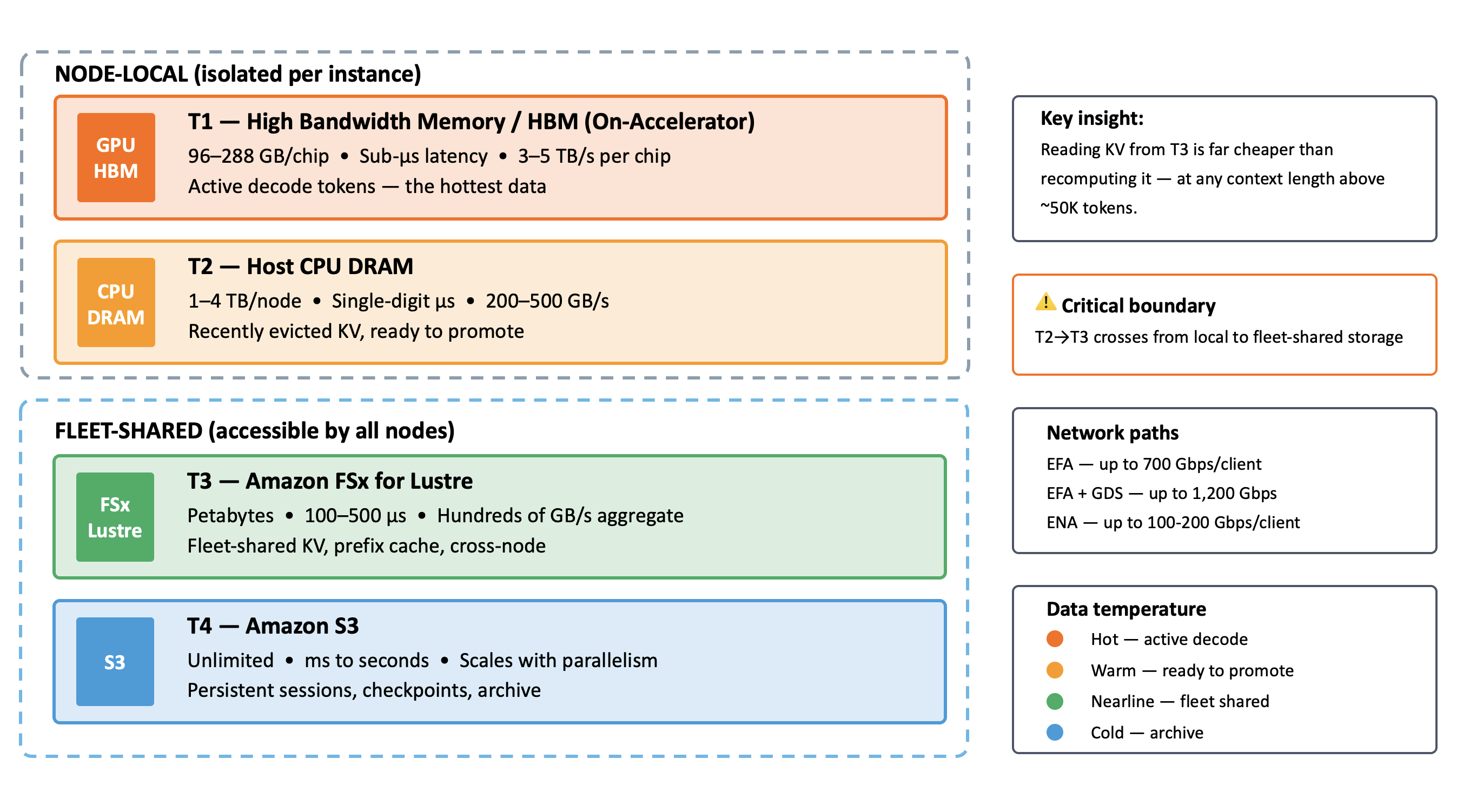
Figure 1: KV cache four-tier storage hierarchy
The following table defines the scope of each tier.
| Tier | Medium | Capacity | Bandwidth | Latency | What lives here |
| T1 | High Bandwidth Memory (HBM) (on-accelerator) | 80–288 GB/chip | 3–8 TBps per chip | Sub-microsecond | Active decode tokens (hot) |
| T2 | Host CPU DRAM | 1–4 TB/node | 200–500 GBps (DDR5) | Single-digit μs | Recently evicted, ready to promote (warm) |
| T3 | Amazon FSx for Lustre | Petabytes | Hundreds of GBps (aggregate) | 100–500 μs | Fleet-shared KV, prefix cache, cross-node (nearline) |
| T4 | Amazon S3 | Unlimited | Scales with request parallelism | milliseconds to seconds | Persistent sessions, checkpoints, archive (frozen) |
Node-local vs. fleet-shared
The tiers have several unique features and applicable use cases:
- T1 and T2 are node-local – They’re fast but isolated. A KV block on Node A’s DRAM is invisible to Node B without additional software coordination.
- T3 provides what node-local tiers can’t – They provide persistence across the fleet and survival beyond instance lifecycle. T3 introduces a shared, high-throughput storage layer accessible by every node simultaneously. This transforms isolated accelerator nodes into a coordinated disaggregated inference system. Specifically:
- Prefix cache sharing – System prompt KV computed one time, read by every node. This avoids redundant prefill across the fleet, directly reducing Time to First Token (TTFT) for cache-hit requests.
- Cross-node KV availability – When new compute spins up or a request lands on a different node, KV is immediately available without recomputation.
- Fleet-wide load balancing – Nodes can pick up sessions from T3, decoupling user affinity from node assignment.
- T4 is durable but offline – It’s too slow for real-time promotion during active decode (seconds when microseconds are needed). Use it for session continuity across hours or days, checkpoints, and archival.
The network data path: Elastic Fabric Adapter and NVIDIA GPUDirect Storage
For a latency-sensitive workload like KV cache promotion, the data path between accelerator memory and storage matters as much as the storage medium itself. One example is Elastic Fabric Adapter (EFA) as the high-bandwidth, low-latency network interface on GPU and Trainium instances. EFA provides both the inter-node fabric (tensor parallelism, KV transfers) and the path to shared storage. When sizing Amazon FSx for Lustre throughput, remember that EFA is shared between compute traffic and storage I/O, so you need to account for both. Another storage option is NVIDIA GPUDirect Storage (GDS), which enables direct DMA transfers between GPU HBM and storage, bypassing CPU and host DRAM entirely. On supported instance types with FSx for Lustre, GDS removes the CPU bounce buffer, keeping the path between T1 and T3 as short as physics allows.
FSx for Lustre delivers up to 100 Gbps per client over ENA, up to 700 Gbps over EFA, and up to 1,200 Gbps over EFA with GDS. That ceiling bounds how many concurrent cache-hit sessions a single node can absorb. GDS is available only on NVIDIA GPU instances. On Trainium, the promotion path from T3 runs over EFA without GDS, so size T3 throughput requirements accordingly.
We recommend planning for and deploying FSx for Lustre in the same Availability Zone as your cluster to minimize latency. GDS requires placement in the same Availability Zone.
Sizing your KV cache footprint
To access a workload and determine how much KV cache storage you need, use the formula: KV bytes per token = 2 × num_layers × num_kv_heads × head_dim × bytes_per_element
The following table summarizes the KV cache sizing variables.
| Variable | What it represents | Where to find it |
| num_layers | Transformer layers (depth) | Model config.json: num_hidden_layers |
| num_kv_heads | KV attention heads; might differ from query heads in Grouped Query Attention (GQA) | Model config.json: num_key_value_heads |
| head_dim | Dimension per head | Model config.json: hidden_size / num_attention_heads |
| bytes_per_element | Precision: FP16/BF16 = 2, FP8 = 1, INT4/TQ = 0.5 | Your serving config |
Real-world examples
Let’s apply the formula to two production-scale models:
- Meta Llama 3.1 405B (GQA, 8 KV heads) – 2 × 126 layers × 8 heads × 128 dim × 2 B = 516 KB (approximately 0.5 MB) per token
- DeepSeek-R1 671B (Mixture of Experts (MoE) + Multi-head Latent Attention (MLA)) – (c_kv_dim + rope_dim) × bytes_per_element × num_layers = (512 + 64) × 2 × 61 = approximately 70 KB per token
MLA caches a low-rank latent instead of full K/V heads, producing a footprint seven times smaller than Llama 3.1 405B despite R1 being the larger model.
Quantization: A complementary lever
The bytes_per_element variable isn’t fixed. KV cache quantization compresses stored vectors from FP16 (2 B) to FP8 (1 B) or INT4 (0.5 B), reducing per-token KV size by 50–75 percent.
Total footprint at scale
The following formula determines the total KV footprint at scale:
Total KV = KV_per_token × context_length × concurrent_sessions
As the following table shows, at the moderate end, 10 TB of live KV might fit in a Trn3 UltraServer’s aggregated HBM. The agent end might contain petabytes. This is the range we’re designing for.
| Scenario | KV/token (BF16 baseline) | Context | Sessions | Total KV | Implication |
| GQA model, moderate | 0.5 MB | 200K | 100 |
|
Fits in Trn3 UltraServer HBM; with TQ, fits with headroom |
| Dense model, moderate | 4 MB | 200K | 100 |
|
Exceeds single node at all precisions; T3 required |
| GQA model, agentic | 0.5 MB | 1M | 500 |
|
Requires fleet-wide tiering |
| Dense model, agentic | 4 MB | 1M | 500 |
|
Multi-tier mandatory |
The UltraServer advantage
Before you assume T3 is always required, it’s worth understanding how the Trn3 UltraServer changes the calculus.
The Trn3 UltraServer aggregates 20.7 TB of HBM3e across 144 Trainium3 chips connected by NeuronLink at 706 TBps. Compare that to a standard 8-GPU node with 1.1-2.3 TB of HBM: a 9–18 times larger Tier 1 pool.
This changes the tiering math substantially:
- Workloads that overflow T1 on an 8-GPU node might fit entirely in T1 on a Trn3 UltraServer.
- When they do overflow, the threshold is higher; less data flows to external tiers, reducing storage I/O requirements.
- Because 20.7 TB of T1 already exceeds what T2 can provide on a standard node, the intermediate tiers add complexity without meaningful capacity benefit. A Trn3 deployment can often go directly from T1 to T3: when KV exceeds HBM, it spills to the fleet-shared tier rather than bouncing through node-local DRAM and NVMe.
The UltraServer doesn’t eliminate tiering at frontier scale. Even 20.7 TB overflows when you hit high concurrency with long contexts. But it raises the bar for when T3 becomes necessary.
The KV data lifecycle
Beyond just knowing which tiers exist, it’s important to know when data should move between them, and what triggers the movement. The following diagram illustrates the states of the KV lifecycle.
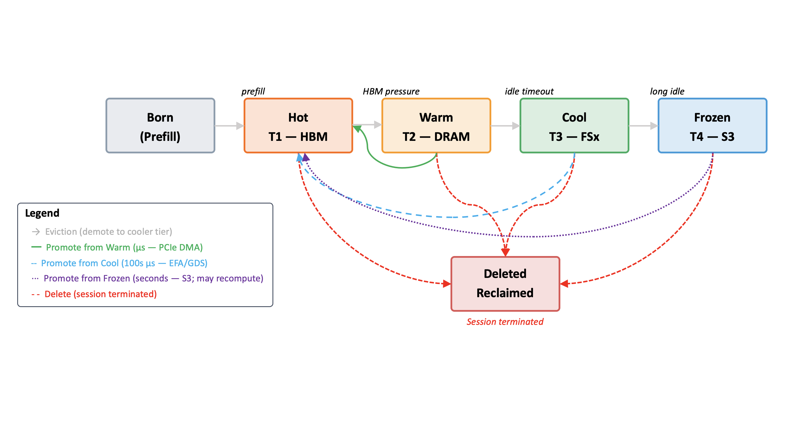
Figure 2: KV block state machine
Eviction policies
A good eviction policy prevents redundant recomputation. The following table lists eviction and movement policies you can tune for your workload.
| Trigger | Action | Rationale |
| HBM pressure > 85% | Evict Least Recently Used (LRU) from T1 to T2 | Protect active decode from stalling |
| Session idle > N seconds | Demote T2 to T3 | Free DRAM for arriving sessions |
| Node-local capacity exceeded | Spill to T3 (Amazon FSx for Lustre) | Node can’t absorb more; fleet storage takes over |
| Session idle > M minutes | Export T3 to T4 (Amazon S3) | Long-idle sessions archived cheaply |
| Session terminated | Delete from all tiers | Reclaim resources immediately |
Eager vs. lazy eviction
You also need to decide how aggressively to evict:
- Eager eviction proactively writes KV to T3 immediately after prefill completes, while keeping a T1 copy for active decode. You get instant recovery on node failure, and immediate availability on any other node, but you double your write bandwidth to T3.
- Lazy eviction keeps KV in T1 until memory pressure forces demotion. This offers lower storage I/O, but if a follow-up request hits a different node, that node has nothing cached and must recompute from scratch.
For disaggregated inference (separate prefill and decode pools), eager eviction is mandatory; the decode node is always different from the prefill node. For non-disaggregated deployments with sticky routing, lazy eviction might work, but consider failure and scale-out scenarios where eager eviction provides resilience.
Promotion policies
When a cache hit arrives for KV that’s already been demoted, you need to bring it back to T1 fast enough that the user doesn’t notice. The following table shows the promotion path from each tier, the mechanism used, and the latency you can expect. This determines whether a cache hit feels instant or whether you’re better off recomputing.
| Cache hit location | Promotion action | Latency |
| T2 | Promote to T1 (DMA over PCIe) | Microseconds, user perceives no delay |
| T3 | Promote to T1 (Amazon FSx for Lustre read) | Hundreds of μs, within TTFT budget for most models |
| T4 | Promote to T1 (Amazon S3 download) | Seconds, might exceed TTFT SLA; consider recompute |
If promotion latency from T4 exceeds the time to rerun prefill, recompute is the better option. For contexts above 50,000 tokens, promotion from T3 is almost always faster than recomputation. For short contexts (under 10,000 tokens), recomputation is inexpensive and tiering adds unnecessary complexity.
Prefix cache namespace design
In most production deployments, a large portion of the KV cache is identical across users: system prompts, Retrieval Augmented Generation (RAG) document preambles, and common instruction templates all produce the same key-value vectors regardless of who’s asking. If every node recomputes that shared prefix independently, you’re spending accelerator time on work that’s already been done. A well-designed prefix cache on T3 avoids this redundancy fleet-wide: compute the prefix one time, store it on shared storage, and let every node read it instead of rerunning prefill.
Shared prefixes benefit from a write-once, read-many pattern on T3:
- Content-addressed naming – Hash the prefix tokens to generate a file path on FSx for Lustre. Use the same prefix, hash, and cache hit, regardless of which node.
- Time-to-live (TTL)-based invalidation – When the system prompt changes, write the new KV with a new hash. Old files expire through TTL.
- Fan-out read pattern – Popular prefixes are read by every node simultaneously. Size FSx for Lustre throughput for this fan-out, not just per-node bandwidth.
Amazon FSx for Lustre as the fleet-shared Tier 4
FSx for Lustre was built for this class of problem: massive parallel throughput, sub-millisecond latency, and shared POSIX access across an entire fleet. For the KV cache use case, it fills the T3 role.
Tier 3 as the parallel file system
T3 has five simultaneous requirements that other storage types don’t meet:
- Shared access from all fleet nodes – The T3 tier must support concurrent reads and writes from every node in the cluster at sub-millisecond metadata latency. This is the design point of a parallel file system, which provides POSIX mounts on every node simultaneously.
- Sub-millisecond read latency – Object storage can’t meet this requirement. FSx for Lustre with SSD backing can.
- Hundreds of GBps aggregate throughput – Block volumes have per-volume limits. A parallel file system stripes across many storage targets, scaling throughput with capacity.
- POSIX file semantics – Inference frameworks (vLLM, SGLang, LMCache) use standard file I/O for KV offload; no SDK integration or custom serialization required.
- Petabyte scale with Amazon S3 lifecycle – FSx for Lustre provides built-in Amazon Simple Storage Service (Amazon S3) data repository association for automatic cold-tier export.
Sizing FSx for Lustre as Tier 3
Now that you know how much KV overflows your node-local tiers, the next question is: how big does your FSx for Lustre file system need to be, and how much throughput should you provision? The answer comes down to three numbers: peak write bandwidth (eviction rate), peak read bandwidth (promotion rate), and total working set capacity. You can determine this through the following steps:
- Determine peak overflow rate (write bandwidth):
- Lazy eviction: (new_sessions/second × KV_per_session) − evictions_returning_capacity/second
- Eager eviction: new_sessions/second × KV_per_session
- Determine peak promotion bandwidth (read bandwidth): cache_hit_rate × requests/second × avg_KV_per_promoted_session.
- Pick your throughput tier. FSx for Lustre offers throughput tiers at 125, 250, 500, and 1,000 MBps per TiB. Choose the tier where: provisioned_capacity_TiB × throughput_per_TiB ≥ max(write_requirement, read_requirement).
- Size capacity for the KV working set. FSx for Lustre capacity = peak_sessions × avg_KV_per_session × (1 − T1_T2_absorption_ratio).
Configuration checklist
When you deploy FSx for Lustre as your T3 tier, several configuration choices affect KV cache performance and cost. It’s important to make the correct choice at provisioning time, because most can’t be changed without rebuilding the file system. The following table summarizes the key settings and our recommendations.
| Setting | Recommendation | Why |
| File system type | Persistent, SSD | Sustained throughput; survives across sessions |
| Availability Zone | Same Availability Zone as cluster | Avoid cross-AZ latency and transfer cost |
| Data compression | Disabled | KV tensors in compact precision; compression adds CPU overhead without meaningful size reduction |
| Amazon S3 Data Repository Association | Enabled | Auto-export cold KV to T4 |
| Lustre client mount options | flock,noatime | Reduce metadata overhead |
| I/O mode | O_DIRECT | Bypass page cache; the inference engine manages its own hierarchy |
| Stripe count | ≥ node count | Distribute I/O across all OSTs |
| I/O worker threads | 32+ per node | Saturate available bandwidth |
Integration with inference frameworks
A tiered storage hierarchy only works if your serving framework knows how to use it. The major inference frameworks support external KV offload, but they each handle it differently. Some manage KV at the page level, some are prefix-aware, and some delegate tier management to an external library. Understanding how your chosen framework interacts with shared storage determines whether integration is a config change or a development effort. The following table summarizes the current landscape.
| Framework | T3 integration | Notes |
| vLLM | KV Block Manager for file system offload | Paged attention; FSx mount as offload target |
| SGLang | RadixAttention with external cache backend | Prefix-aware; natural fit for shared prefix on FSx |
| LMCache | Native file system backend | Purpose-built for external KV; handles serialization and deduplication |
| NVIDIA Dynamo | KVBM multi-tier config | Supports HBM, DRAM, and FS tier chain |
| llm-d (Amazon EKS) | Shared Persistent Volume Claim (PVC) backed by FSx for Lustre | Prefill and decode pods share KV through mounted volume |
Disaggregated inference
In disaggregated inference, T3 becomes architecturally mandatory. The idea is straightforward: separate prefill (compute-bound, GPU-hungry) from decode (memory-bound, latency-sensitive) into independent pools that scale independently. You get hardware specialization, better utilization, and the ability to scale each phase without over-provisioning the other. But it creates a hard data transfer problem: KV generated on Prefill Node A must reach Decode Node B, and those two nodes might never have communicated before.
The following figure shows how T3 solves this by providing an any-to-any data plane between the two pools.
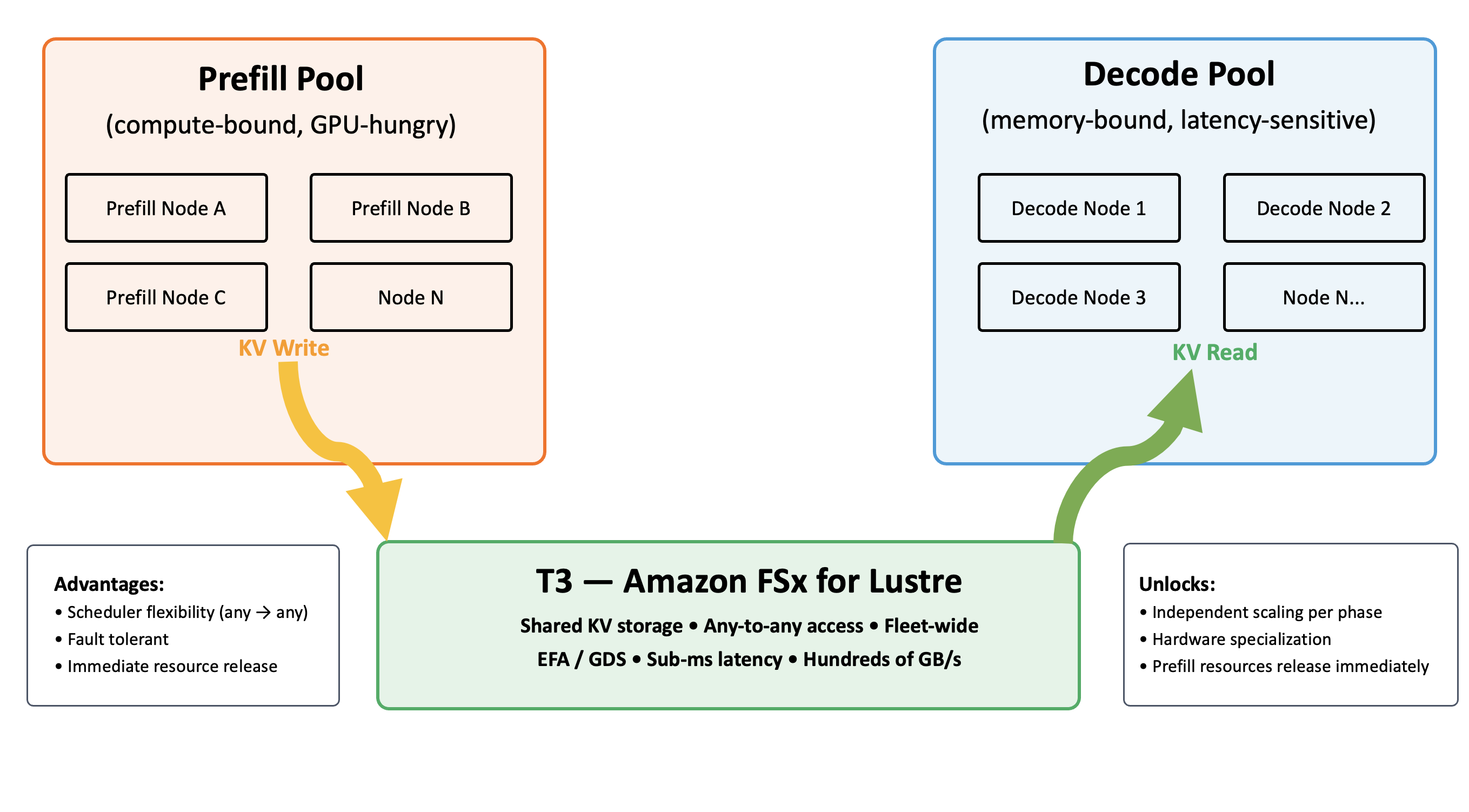
Figure 3: Disaggregated inference with shared T3 storage
Without shared storage, the scheduler must pre-select the decode node before prefill starts (coupling the two pools), or perform a large point-to-point transfer after prefill (added latency). Decode node failure means rerunning prefill entirely.
With FSx for Lustre as T3, prefill nodes write KV to FSx, and a decode node reads it. The scheduler gets full flexibility. In the case of node failure, another decode node picks up the KV from the shared tier. Prefill resources release immediately after write.
The I/O pattern is predictable: large sequential writes at prefill completion, large sequential reads at decode start. The parallel striping in FSx for Lustre handles both natively.
When to deploy this architecture
In this post, we’ve covered the framework end-to-end: tiers, sizing, lifecycle, shared storage, and disaggregated inference. However, not every workload needs all four tiers.
Deploy T3 in the following scenarios:
- Your KV working set regularly exceeds fleet-wide HBM capacity
- More than 30 percent of requests share common prefixes
- Average session idle time exceeds 30 seconds
- You’re adding accelerator nodes primarily to hold KV rather than to serve active decode
- Peak-to-average concurrency ratio exceeds three times greater
- You’re adopting disaggregated inference with separate prefill and decode pools
T3 might not be needed when in the following cases:
- Short context (under 10,000 tokens) with low concurrency: T1 alone is sufficient
- Medium context (10,000–100,000) with moderate concurrency: T1 and T2 might suffice
Getting started
The following steps are a practical path from profiling to production:
- Measure KV per token for your model (use the formula provided earlier). Measure concurrency patterns, prefix overlap ratio, and session idle distribution.
- Use the sizing methodology to determine T3 throughput and capacity.
- Create a Persistent SSD FSx for Lustre file system in the same Availability Zone as your cluster.
- Install the Lustre client on all inference nodes. Set O_DIRECT, 32+ I/O threads, stripe-aligned I/O.
- Configure your framework (vLLM, SGLang, LMCache, Dynamo, or llm-d) to use the FSx mount as the external KV tier.
- Configure lifecycle policies with eviction thresholds, promotion triggers, prefix cache TTLs, and Amazon S3 export schedules.
- Track T1 utilization, T3 cache-hit rate, promotion latency (TTFT on cache-hit vs. miss), and FSx throughput saturation.
Clean up
Delete the test infrastructure when evaluation is complete. If you provisioned FSx for Lustre for testing, delete the file system and resources from the Amazon FSx console to avoid ongoing charges by following these steps:
- Unmount the file system on each compute instance:
sudo umount /mnt/fsx - On the Amazon FSx console, select the file system, choose Actions, then choose Delete file system. Alternatively, run the following command to delete the FSx for Lustre file system:
aws fsx delete-file-system --file-system-id fs-xxxxxxxx - Remove the data repository association (if you configured Amazon S3 export) before deleting, or confirm it is removed with the file system.
- Delete the security group rules you created for Lustre client traffic (ports 988/1018–1023).
- Terminate test compute instances you launched specifically for the evaluation.
Conclusion
Inference performance begins beyond the GPU. This post showed how to keep your fleet working from stored state instead of recomputing it, by sizing your KV cache, organizing it across four tiers, and using FSx for Lustre as the shared layer that connects them all. If you’re running inference at scale, you’re paying for KV recomputation: every time a user returns to an idle session, a request lands on the wrong node, or a popular system prompt gets prefilled redundantly across your fleet. This framework gives you the tools to reduce that cost.
Reading KV from shared storage is frequently cheaper than recomputing it. To build your architecture, size your footprint, tier your data by temperature, and let FSx for Lustre serve as the fleet-wide shared layer that connects it all.
You don’t have to implement all four tiers from the start. Start by profiling your model’s KV per token and measuring your peak concurrency. If the numbers show you’re overflowing a single node (and at production concurrency, they almost certainly will), deploy an FSx for Lustre file system in the same Availability Zone as your cluster, point your inference framework at it, and watch your cache-hit ratio climb while your per-token cost drops.
To learn more about inference storage architecture for your workload, refer to the Amazon FSx for Lustre User Guide and Trn3 UltraServer specifications, or contact your AWS account team.