AWS Big Data Blog
Develop an application migration methodology to modernize your data warehouse with Amazon Redshift
Data in every organization is growing in volume and complexity faster than ever. However, only a fraction of this invaluable asset is available for analysis. Traditional on-premises MPP data warehouses such as Teradata, IBM Netezza, Greenplum, and Vertica have rigid architectures that do not scale for modern big data analytics use cases. These traditional data warehouses are expensive to set up and operate, and require large upfront investments in both software and hardware. They cannot support modern use cases such as real-time or predictive analytics and applications that need advanced machine learning and personalized experiences.
Amazon Redshift is a fast, fully managed, cloud-native and cost-effective data warehouse that liberates your analytics pipeline from these limitations. You can run queries across petabytes of data in your Amazon Redshift cluster, and exabytes of data in-place on your data lake. You can set up a cloud data warehouse in minutes, start small for just $0.25 per hour, and scale to over a petabyte of compressed data for under $1,000 per TB per year – less than one-tenth the cost of competing solutions.
With tens of thousands of current global deployments (and rapid growth), Amazon Redshift has experienced tremendous demand from customers seeking to migrate away from their legacy MPP data warehouses. The AWS Schema Conversion Tool (SCT) makes this type of MPP migration predictable by automatically converting the source database schema and a majority of the database code objects, including views, stored procedures, and functions, to equivalent features in Amazon Redshift. SCT can also help migrate data from a range of data warehouses to Amazon Redshift by using built-in data migration agents.
Large-scale MPP data warehouse migration presents a challenge in terms of project complexity and poses a risk to execution in terms of resources, time, and cost. You can significantly reduce the complexity of migrating your legacy data warehouse and workloads with a subject- and object-level consumption-based data warehouse migration roadmap.
AWS Professional Services has designed and developed this tool based on many large-scale MPP data warehouse migration projects we have performed in the last few years. This approach is derived from lessons learned from analyzing and dissecting your ETL and reporting workloads, which often have intricate dependencies. It breaks a complex data warehouse migration project into multiple logical and systematic waves based on multiple dimensions: business priority, data dependency, workload profiles and existing service level agreements (SLAs).
Consumption-based migration methodology
An effective and efficient method to migrate an MPP data warehouse is the consumption-based migration model, which moves workloads from the source MPP data warehouse to Amazon Redshift in a series of waves. You should run both the source MPP data warehouse and Amazon Redshift production environments in parallel for a certain amount of time before you can fully retire the source MPP data warehouse. For more information, see How to migrate a large data warehouse from IBM Netezza to Amazon Redshift with no downtime.
A data warehouse has the following two logical components:
- Subject area – A data source and data domain combination. It is typically associated with a business function, such as sales or payment.
- Application – An analytic that consumes one or more subject areas to deliver value to customers.
The following diagram illustrates the workflow of data subject areas and information consumption.
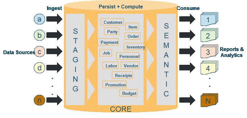
Figure 1: Consuming applications (reports/analytics) and subject areas (data source/domain).
This methodology helps to facilitate a customer’s journey to build a Data Driven Enterprise (D2E). The benefits are: 1) helping to deeply understand the customer’s business context and use-cases and 2) contributing to shaping an enterprise data migration roadmap.
Affinity mapping between subject area and application
To decide which applications and their associated subject areas go into which wave, you need a detailed mapping between applications and subject areas. The following table shows an example of this type of mapping.

Figure 2: The affinity mapping between applications (analytics) and subject areas.
The basis for this mapping is the query execution metadata often stored in system tables of legacy data warehouses. This mapping is the basis for the creation of each wave — a single-step migration of an application’s objects and associated subject areas. You can similarly derive another potential second step, which results in a more detailed mapping between data sources and subject areas (to the level of individual tables) and helps with detailed project planning.
The sorting method in the preceding table is important. The right-most column shows the total number of times a subject area appears in applications (from the most common subject area to the least common subject area, top to bottom). The bottom row displays the number of subject areas that appear in an application (from the most dense application to the least dense, from left to right).
Given all other conditions being equal, which applications and analytics should you start with for the first wave? The best practice is to start somewhere in the middle (such as Analytic 8 or 9 in the preceding table). If you start from the left-most column (Analytic 1), the wave includes numerous objects (sources and tables, views, ETL scripts, data formatting, cleansing and exposing routines), which makes it unwieldy and inordinately long to execute and complete. Alternatively, if you start from the right-most column (Analytic 19), it covers very few subject areas and increases the number of waves required to complete the entire migration to a longer time frame. This choice also fails to offer good insight into the complexity of the whole project.
Migration wave and subject area integration
The following table illustrates the wave-based migration approach (stair steps) for the preceding affinity map. In each wave (which may include one or more applications or analytics), there are always new subject areas (in green) to onboard and subject areas that were migrated in the previous waves (in blue). An optimal wave-based migration approach is to design migration waves to have fewer new builds with each subsequent wave. In the following example, as earlier waves finish, there are fewer new subject areas to integrate in the subsequent waves — another reason to start in the middle and work to the left on the affinity chart. This ultimately results in accelerated delivery of your migration outcomes.

Figure 3: Stair step model and subject area integration.
Wave 0 typically includes the shared or foundational dimensional data or tables that every application uses (for example, Time and Organization). Each wave should have at least one anchor application, and anchor applications need to include new subject areas or data sources. What factors should you consider when choosing anchor applications in a wave? An anchor application in one wave should have minimal dependencies on other anchor applications in other waves, and it is often considered important from the business perspective. The combination of anchor applications across all waves should cover all subject areas.
In the preceding example, there are six different migration waves. The following table summarizes their anchor applications:
| Migration Wave | Anchor Applications |
| Wave 1 | Analytic 9 |
| Wave 2 | Analytic 8 |
| Wave 3 | Analytic 7 |
| Wave 4 | Analytic 6 |
| Wave 5 | Analytic 4 and Analytic 5 |
| Wave 6 | Analytic 3 |
All the other applications (analytics) will be automatically taken care of because the subject areas they are dependent upon will have already been built in the above mentioned waves.
Application onboarding best practices
To determine how many waves there should be and what applications should go into each wave, consider the following factors:
- Business priorities – An application’s value as part of a customer’s Data Driven Enterprise (D2E) journey
- Workload profiles – Whether a workload is mostly ETL (write intensive) or query (read only)
- Data-sharing requirements – Different applications may use data in the same tables
- Application SLAs – The promised performance metric to end-users for each application
- Dependencies – Functional dependencies among different applications
The optimal number of waves is determined based on the above criteria, and the best practice is to have up to 10 waves in one migration project so that you can effectively plan, execute and monitor.
Regarding what applications should go into which wave and why, interactions among applications and their performance impact are typically too complex to understand from first principles. The following are some best practices:
- Perform experiments and tests to develop an understanding about how applications interact with each other and their performance impact.
- Group applications based on common data-sharing requirements.
- Be aware that not all workloads benefit from a large cluster. For example, simple dashboard queries may run faster on small clusters, while complex queries can take advantage of all the slices in a large Amazon Redshift cluster.
- Consider grouping applications with different workload and access patterns.
- Consider using a dedicated cluster for different waves of applications.
- Develop a workload profile for each application.
Amazon Redshift cluster sizing guide
The Amazon Redshift node type determines the CPU, RAM, storage capacity, and storage drive type for each node. The RA3 node type enables you to scale compute and storage independently. You pay separately for the amount of compute and Amazon Redshift Managed Storage (RMS) that you use. DS2 node types are optimized to store large amounts of data and use hard disk drive (HDD) storage. If you currently run on DS2 nodes, you should upgrade to RA3 cluster to get up to 2x better performance and 2x more storage for the same cost. The dense compute (DC) node types are optimized for compute. DC2 node types are optimized for performance-intensive workloads because they use solid state drive (SSD) storage.
Amazon Redshift node types are available in different sizes. Node size and the number of nodes determine the total storage for a cluster. We recommend 1) if you have less than 1TB of compressed data size, you should choose DC2 node types; 2) for more than 1TB of compressed data size choose RA3 node types (RA3.4xlarge or RA3.16xlarge). For more information, see Clusters and Nodes in Amazon Redshift.
The node type that you choose depends on several factors:
- The compute needs of downstream systems to meet Service Level Agreements (SLAs)
- The complexity of the queries and concurrent operations that you need to support in the database
- The trade-off between achieving the best performance for your workload and budget
- The amount of data you want to store in a cluster
For more detailed information about Amazon Redshift cluster node type and cluster sizing, see Clusters and nodes in Amazon Redshift.
As your data and performance needs change over time, you can easily resize your cluster to make the best use of the compute and storage options that Amazon Redshift provides. You can use Elastic Resize to scale your Amazon Redshift cluster up and down in a matter of minutes to handle predictable spiky workloads and use the automated Concurrency Scaling feature to improve the performance of ad-hoc query workloads.
Although you may be migrating all the data in your traditional MPP data warehouses into the managed storage of Amazon Redshift, it is also common to send data to different destinations. You might send cold or historical data to an Amazon S3 data lake to save costs, and send hot or warm data to an Amazon Redshift cluster for optimal performance. Amazon Redshift Spectrum allows you to easily query and join data across your Amazon Redshift data warehouse and Amazon S3 data lake. The powerful serverless data lake approach using AWS Glue and AWS Lambda functions enables the lake house architecture that combines data in an Amazon S3 data lake with data warehousing in the cloud using a simplified ETL data pipeline, minimizing the need to load data into an Amazon Redshift cluster. For more detailed information, see ETL and ELT design patterns for lake house architecture using Amazon Redshift: Part 1 and Build and automate a serverless data lake using an AWS Glue trigger for the Data Catalog and ETL jobs.
Conclusion
This post demonstrated how to develop a comprehensive, wave-based application migration methodology for a complex project to modernize a traditional MPP data warehouse with Amazon Redshift. It provided best practices and lessons learned by considering business priority, data dependency, workload profiles and existing service level agreements (SLAs).
We would like to acknowledge AWS colleagues Corina Radovanovich, Jackie Jiang, Hunter Grider, Srinath Madabushi, Matt Scaer, Dilip Kikla, Vinay Shukla, Eugene Kawamoto, Maor Kleider, Himanshu Raja, Britt Johnston and Jason Berkowitz for their valuable feedback and suggestions.
If you have any questions or suggestions, please leave your feedback in the comment section. For more information about modernizing your on-premises data warehouses by migrating to Amazon Redshift and finding a trusted AWS partner who can assist you on this endeavor, see Modernize your Data Warehouse.
About the authors
 Po Hong, PhD, is a Principal Data Architect of Data & Analytics Global Specialty Practice, AWS Professional Services.
 Anand Rajaram is the global head of the Amazon Redshift Professional Services Practice at AWS.