AWS Database Blog
Store and analyze time-series data with multi-measure records, magnetic storage writes, and scheduled queries in Amazon Timestream
Time series is one of the most common data formats, particular when collecting information from applications, infrastructure, and IoT devices. Amazon Timestream is a serverless time series database that scales with your data and makes it easy to store and analyze your events at a much lower cost than relational databases. During AWS re:Invent 2021, Timestream announced new updates that make it easier and cheaper to implement many use cases:
- Multi-measure records – You can now include more than one measure in a Timestream record. This makes it easy to load your data and reduces the number of records to write and query for many use cases. For example, you can use multi-measure records when you’re tracking more than one metric emitted from the same source at the same time. Multi-measure records also simplify migrating data from relational databases to Timestream because the database schema needs fewer or no changes.
- Magnetic storage writes – Timestream manages the lifecycle of your data with storage tiers: a memory store for recent data and a magnetic store for historical data. The transfer of data from the memory store to the magnetic store is automated and based on configurable policies. Previously, data could only be loaded to the memory store. Now, you can optimize storage costs by sending late-arriving data to the magnetic store instead of keeping a large memory store.
- Scheduled queries – You can point dashboards and reports to a table containing the result of a scheduled query instead of querying directly the source table. For example, if you’re running frequent aggregates in your queries, such as sums and averages over a large dataset, you can now materialize these results into another table for lower latency and cost.
Let’s see how to use these new capabilities by applying them to a use case. In this post, we show how to use multi-measure records to simplify the data format of an existing database, enable magnetic storage writes to manage late-arriving data, and implement scheduled queries to improve performance and reduce costs for dashboards and reports.
Simplify the data format with multi-measure records
In the announcement of the general availability of Timestream, we built a simple IT monitoring application collecting CPU, memory, swap, and disk usage from a server. These four measurements were each written into their own record using a data model we call single-measure records. Now, with multi-measure records, these four measurements can be ingested, stored, and queried together because they’re emitted at the same time.
While collecting data, each server is identified by a host name and a location expressed as a country and a city. For this use case, the dimensions used to categorize data are the same for all records:
countrycityhostname
There are four measures to collect:
cpu_utilizationmemory_utilizationswap_utilizationdisk_utilization
To create a new Timestream database and table, we use the following AWS CloudFormation template:
We create the stack with the AWS Command Line Interface (AWS CLI):
When the stack is ready, we update the application to load data using the multi-measure records. Previously, for each timestamp, we had to insert four records, one for each measure. Now, we can collect all measures at the same time and store them in one record.
The following is the Python code for the updated collect.py application:
In the code, we set a measure name for the whole record (we use utilization) and use the MULTI measure value type. Then we can add multiple measure values, each with their name, value, and type.
To run the application, we use this run.sh script using the AWS CLI to fill the DATABASE_NAME and TABLE_NAME environment variables with the outputs of the CloudFormation stack:
We start the script on a laptop to collect some meaningful usage data. Measures are written to the Timestream table in batches of 100 records. Each record contains a single timestamp and four measures (CPU, memory, disk, swap):
On the Timestream console, we run a query to see the last few records inserted in the table.
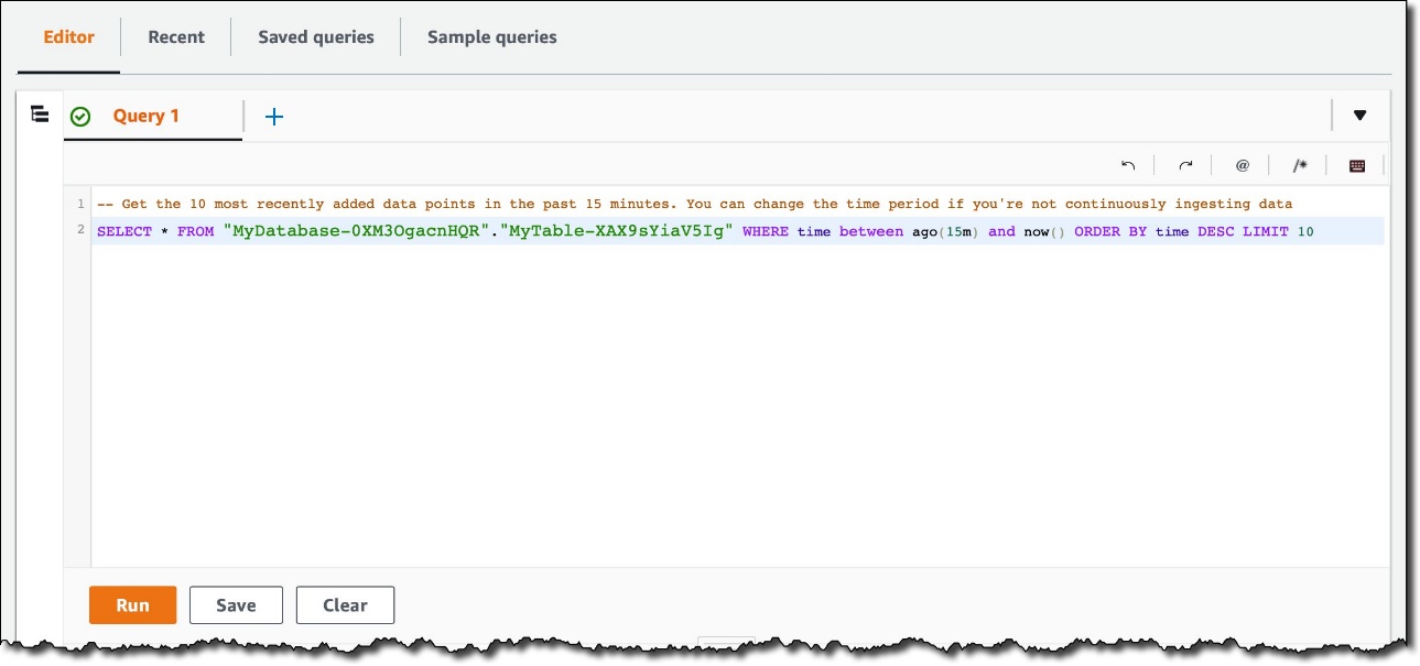
The following screenshot shows the records using the new multi-measure format. As expected, each record has the three dimensions used to categorize the data (hostname, city, and country), a time, a measure_name equal to utilization, and four measures with their values: cpu, memory, disk, and swap.

With multi-measure records, we reduce the number of records written and stored in the table. Previously, for each timestamp, we were writing four records, one for each measure. Now, we write the four measures emitted at the same time in one multi-measure record. We also use less storage, but we have the same level of information as before.
Running queries on multi-measure records is easier and more efficient because less data needs to be processed. For example, we don’t need to use joins to return multiple measures with the same query. This also reduces our overall costs.
Manage late-arriving data and data corrections with magnetic storage writes
When working with time series, you have to manage late-arriving data, which is data with a timestamp that is in the past. There can be many reasons why you receive late-arriving data and they’re often outside of your control. For example, an application or a device might be stopped or disconnected from the network for some time and is going to send all buffered data at once when it’s back online.
Previously with Timestream, you had to increase the memory store retention of your table to accept late arrivals. That’s because data outside of the memory retention period was rejected when you tried to write it into a table.
Now, you can send late-arriving data to the magnetic store by simply enabling a property on your tables. You use the same WriteRecord API call to write data to Timestream. Depending on the timestamp on the data point and the table’s configured memory store retention, the data is automatically routed to the appropriate store.
With this feature, you can now right-size your memory store data retention period to match your data ingestion throughput and the query requirements of your application. Magnetic store writes are applied asynchronously, so the data written cannot be immediately queried. However, the data is durable for any write request which the system has acknowledged.
For the IT monitoring application, when network issues occur in remote locations, data can be sent that is a few days old. Memory retention for the table is currently 24 hours (see the MemoryStoreRetentionPeriodInHours property in the CloudFormation template used to create the table).
To store data that is older than 1 day, on the Timestream console, we select our table and choose Edit. Under Data Retention options, there is the new Magnetic Storage Writes section. We enable the setting and add a location on Amazon Simple Storage Service (Amazon S3) for the error logs. It’s important to add a location for the logs because magnetic storage writes are asynchronous and you don’t have another way to get feedback if some records can’t be written (for example, because there is a version mismatch).

Improve performance and reduce costs for dashboards and reports with scheduled queries
To further optimize costs, we can use a scheduled query to prepare the data we use more frequently for reports and dashboards. For example, we previously created a Grafana dashboard for the IT monitoring application. We connected the Timestream table as data source and used the following query to collect data for the dashboard ($__database and $__table are macros defined by the data source):
The following screenshot shows our output:

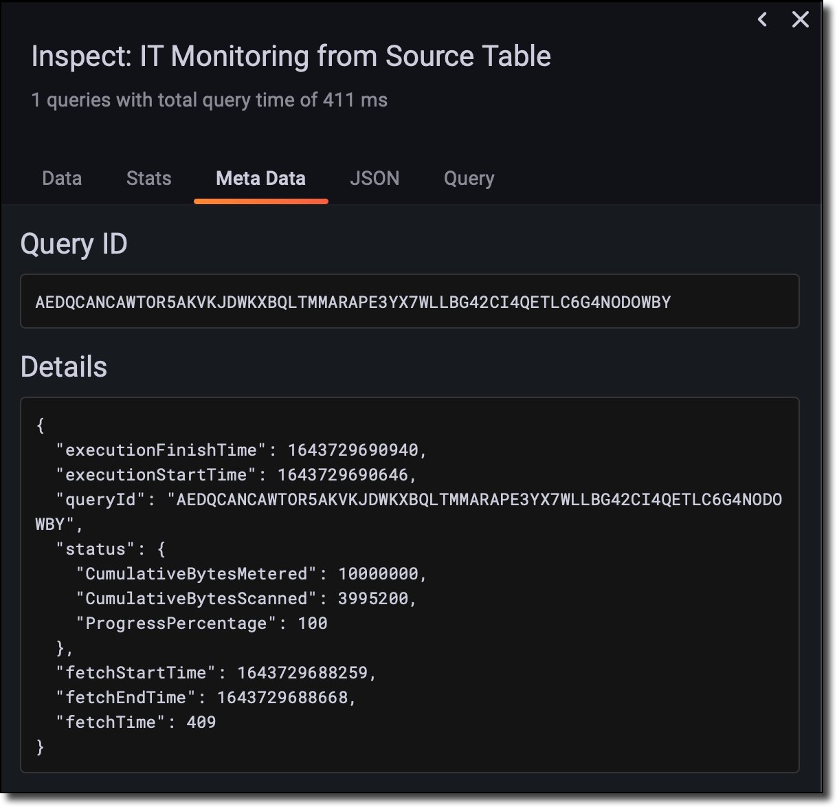
To understand how the query is run by Timestream, we inspect the query metadata.

In the query metadata, we see that about 4 MB has been scanned by Timestream (CumulativeBytesScanned) to populate the dashboard with a latency of 400 milliseconds (fetchTime). The amount of data scanned is affecting both the cost and the performance of the query.
To optimize costs and improve performance, we can configure a scheduled query to populate another table with pre-aggregated data. Then we can point dashboards and reports to this new table instead of querying the considerably larger source table.
First, we create a table to store the result of the scheduled query. To do so, we add a new resource to the CloudFormation template:
Then, using the AWS CLI, we update the CloudFormation stack:
In the Timestream console, we create a scheduled query. We select the new table as the destination and enter a name for the scheduled query. We can also create scheduled queries using CloudFormation but following the process in the console makes it easier to understand how they work.

In the Query statement section, we use the following SQL query to aggregate data in 10-minute intervals. The source table has data with 1-second intervals.

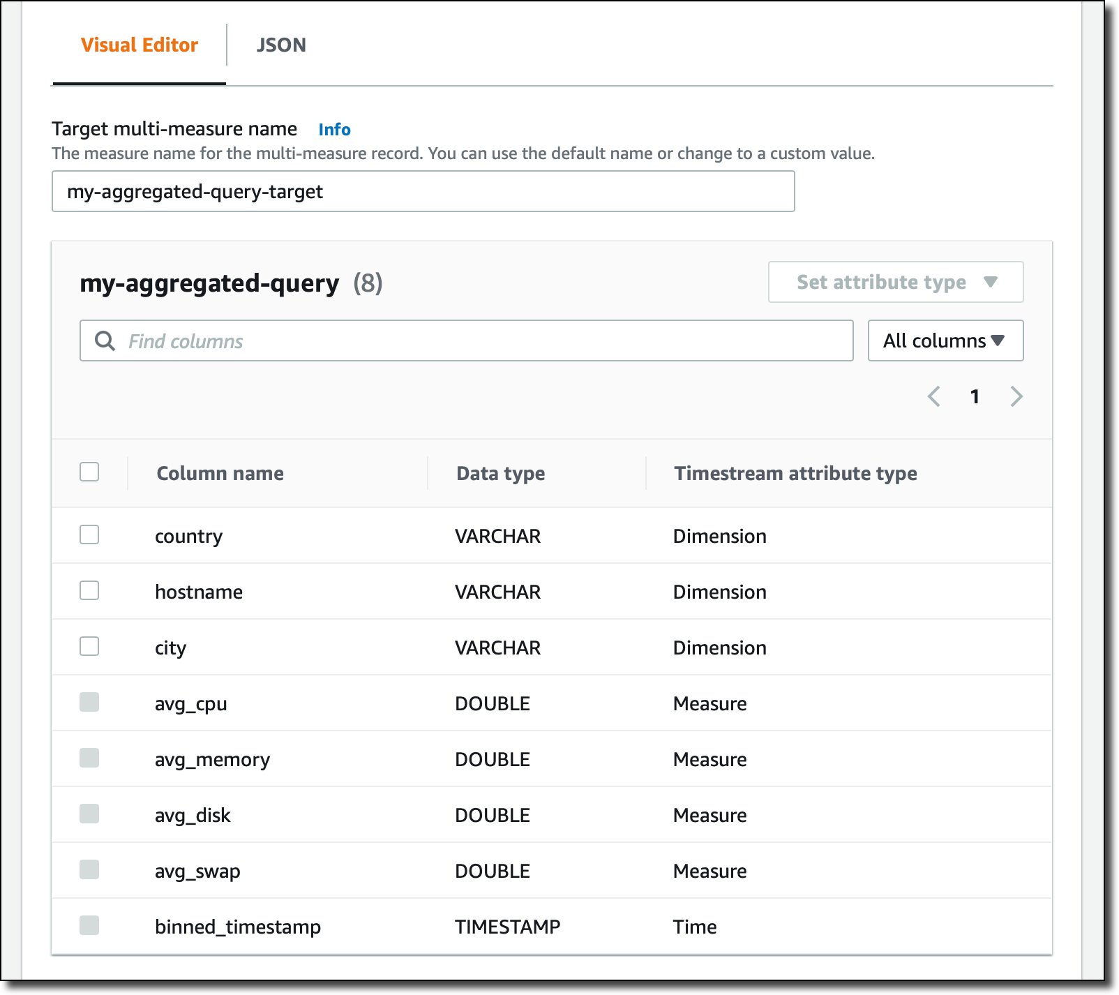
We check that the query is correct by choosing Validate. Then, in the Visual Editor, we leave the default measure name for the multi-measure record and set the attribute type of country, host name, and city to Dimension.
We choose to run the query every 10 minutes. Depending on your use case, you can pick a shorter or longer interval, or use a CRON expression to avoid running the query outside of your business hours.

In the security settings, we choose an AWS Identity and Access Management (IAM) role that we prepared earlier.
The role has three policies attached:
- Timestream permissions to read from the source table and write to the destination table:
- Amazon SNS permissions to publish to the selected SNS topic:
- Amazon S3 permissions to write logs to an S3 bucket:
Finally, the following trust relationship allows Timestream to assume the role:
The role also gives permissions to do the following:
- Publish to an Amazon Simple Notification Service (Amazon SNS) topic to receive a notification when a query runs
- Write logs to an S3 bucket

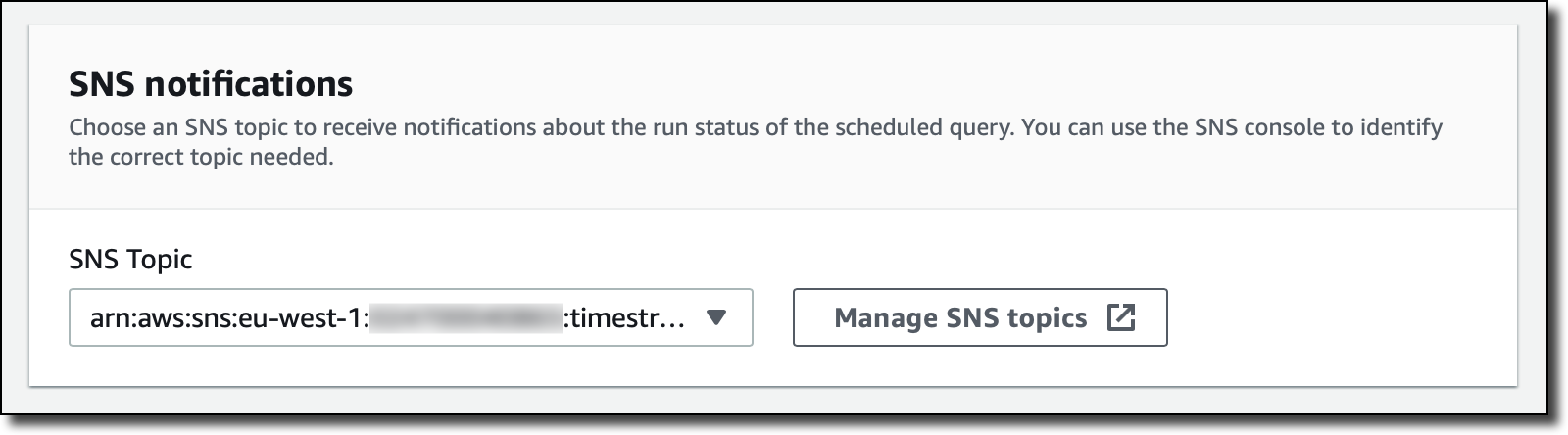
We use the default AWS Key Management Service (AWS KMS) key to encrypt the query statement. Under SNS notifications, we select the SNS topic for the notifications. These notifications are important because they tell you if the scheduled query ran correctly or if an error occurred.
We configure the error report logging to store error logs in an S3 bucket.

Optionally, we can add tags to search and filter resources or track AWS costs. Finally, we review all the configurations and create the scheduled query.
After the scheduled query runs at least once, we create a new dashboard pointing to the aggregated data table. We use the same query as before. We just renamed the measure fields, for example cpu is now avg_cpu, and so on. The result of the query is exactly the same as before.

To see the benefits of using the aggregated table, we review the query metadata again.

About 9 KB has been scanned for the query used to draw the same chart, down from 4 MB when running the query on the source table. The fetch time has also improved, down to 250 milliseconds from 400 milliseconds. As the amount of data stored in the database grows, we will start to see more latency improvements. In this way, the dashboard is faster to render and cheaper to run. For more usage patterns with end-to-end examples of how to use scheduled queries, see Scheduled Query Patterns and Examples.
Clean up
To avoid future costs, we remove all the resources created for this post. First, we delete the CloudFormation stack with the following command. This deletes the database and the two tables.
On the Timestream console, we select the scheduled query and choose Delete on the Actions menu. You can also create scheduled queries using CloudFormation to manage all your Timestream resources as code.

Conclusion
Multi-measure records, magnetic storage writes, and scheduled queries make it easier and cheaper to store and analyze time series data for your applications and are available in all AWS Regions where Timestream is offered.
There are no additional costs for using these new features—in fact, they can all help you optimize your costs. Running scheduled queries means you pay the cost to run the query and then materialize the results. However, if you’re repeatedly loading your dashboards, the cost savings from querying the precomputed results usually is more significant that the cost to run the queries.
Timestream provides the flexibility to model your data in different ways to suit your application’s requirements. For patterns and guidelines for you to optimize your costs and performance, we added a new Data Modeling section in the Timestream documentation. Let us know in the comments or on Twitter what you’re going to build with these new features!
About the Authors
 Danilo Poccia works with startups and companies of any size to support their innovation. In his role as Chief Evangelist (EMEA) at Amazon Web Services, he leverages his experience to help people bring their ideas to life, focusing on serverless architectures and event-driven programming, and on the technical and business impact of machine learning and edge computing. He is the author of AWS Lambda in Action from Manning.
 Sreenath Gotur is a Sr. Timestream Specialist Solutions Architect at AWS based out of Charlotte,NC. Prior to joining AWS, he was heading enterprise data management, enterprise data services and data innovation portfolio with a large Financial firm. Sreenath has a special interest in Data & Analytics, Document DB and Graph DB. In his spare time, he enjoys spending quality time with his family.