AWS Database Blog
Analyze database performance with Amazon CloudWatch metric streams
February 9, 2024: Amazon Kinesis Data Firehose has been renamed to Amazon Data Firehose. Read the AWS What’s New post to learn more.
With the announcement of Amazon CloudWatch Metric Streams, you can now stream near-real-time metrics data to a destination such as Amazon Simple Storage Service (Amazon S3). Metric Streams supports two primary use cases:
- Third-party providers – You can stream metrics to partners to power dashboards, alarms, and other tools that rely on accurate and timely metric data.
- Data lakes – You can send metrics to your data lake on AWS, such as Amazon S3. Streaming metrics to a data lake enables you to retain 1-minute granularity performance for specific events or periods of the year for as long as you want, and then compare this data on a year over year, month over month, or week over week basis.
In this post, we use Metric Streams to continuously ingest monitoring data for a range of database types, at large scale, for long-term metric retention into a data lake on Amazon S3. We then use Amazon Athena to query the data lake to get insights into resource performance and utilization.
We can use other tools such as Performance Insights to analyze and tune Amazon Relational Database Service (Amazon RDS) database performance, which lets you retain Amazon RDS metrics data for a specific time period. However, if you need a centralized way to monitor and troubleshoot different databases at large scale, this post is for you. Not only can you monitor past events over a longer time period, but you can also track the performance and usage of multiple databases from a single point in near-real time. It also works well at scale.
Architecture overview
This following architectural diagram gives a quick summary of how this feature works and how you can use it with other AWS services.
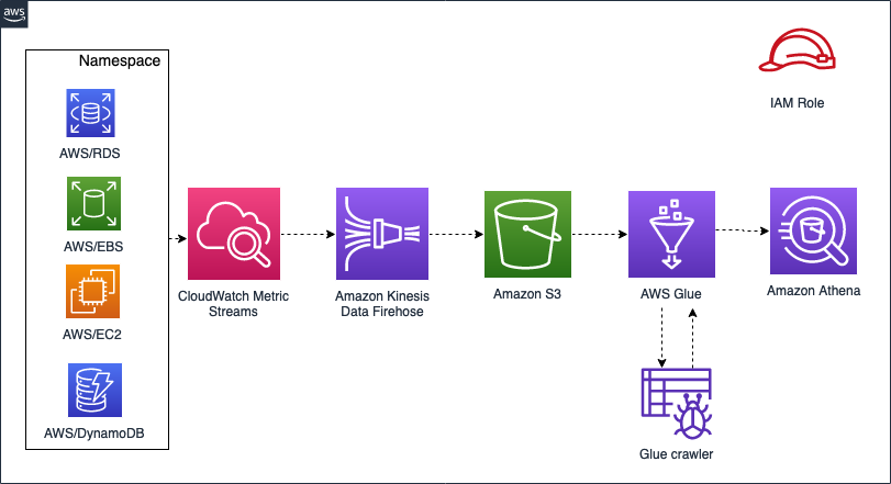
We create an Amazon CloudWatch metrics stream for four different service namespaces: AWS/RDS, AWS/EC2, AWS/EBS, and AWS/DynamoDB. In some use cases, you may have installed databases like MongoDB or MySQL on Amazon Elastic Compute Cloud (Amazon EC2), so you want to monitor underlying host metrics. For that reason, we use Amazon EC2 and Amazon Elastic Block Store (Amazon EBS) namespaces in addition to database service namespaces (Amazon RDS and Amazon DynamoDB).
We use Amazon Kinesis Data Firehose to deliver the metric data to our destination (Amazon S3). When we have metric data flowing in our S3 bucket, we create an AWS Glue database and table with that S3 bucket as the data source. We then use Athena to run queries and analyze the metrics data.
Create a CloudWatch metric stream
To create your stream of CloudWatch metrics, complete the following steps:
- On the CloudWatch console, expand Metrics in the navigation pane. Choose Streams.
- Choose Create metric stream.
- Choose the CloudWatch metric namespaces to include in the metric stream. For this post, we use the following:
- AWS/RDS
- AWS/EC2
- AWS/EBS
- AWS/DynamoDB
- Choose Quick S3 setup.
CloudWatch creates all the necessary resources, including the Kinesis Data Firehose delivery stream and the necessary AWS Identity and Access Management (IAM) roles. The default output format for this option is JSON.
If you already have a Firehose delivery stream that you want to use, you can do so by selecting Select an existing Firehose owned by your account. Similarly, you can either choose an existing IAM role or create a new one.
- For Metric stream name, enter a unique name.
- Choose Create metric stream.
Add a Kinesis Data Firehose delivery stream custom prefix
In this step, we add a custom prefix to our delivery stream to group data by date. This provides the ability to create Glue table partitions by year, month, day and hour. This will control the amount of data scanned by each query using Athena, thus improving performance and reducing cost.
- On the Kinesis Data Firehose console, choose the delivery stream you created.
- Choose Edit.
- In the Amazon S3 destination section, for Backup S3 bucket prefix, enter
- For Backup S3 bucket error prefix, enter
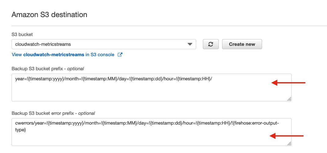
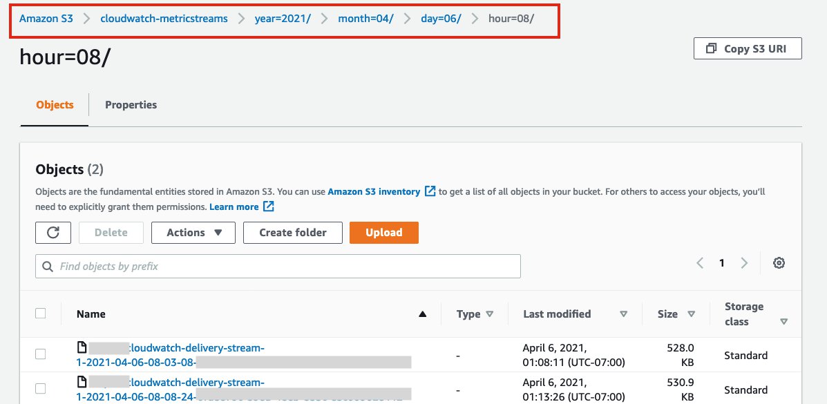
After updating, you may have files created using the previous default naming convention, which you should delete. After you delete the files that were stored on S3 prior to adding the delivery stream prefix, you can see the new files coming in following the newly specified naming convention.
Adding the prefix sets the Amazon S3 location in which the data records are delivered (for example, year=2021/month=04/day=06/hour=08/).
Set up an AWS Glue database, crawler, and table
You should now have your CloudWatch metrics stream configured and metrics flowing to your S3 bucket. In this step, we configure the AWS Glue database, crawler, table, and table partitions.
- On the AWS Glue console, choose Add database.
- Enter a name for your database, such as
cloudwatch_metricstreams_db.
Now that we have our AWS Glue database in place, we set up the crawler.
- In the navigation pane, choose Crawlers.
- Choose Add crawler.
- Enter a name for your crawler, such as
cloudwatch_metricstreams_crawler. - Choose Next.
- For Add a data store, choose S3.
- For Include path, enter the S3 path to the folders or files that you want to crawl.
- Choose Next.
- For Add another data store, choose No.
- For Choose IAM role, choose an existing role with the necessary permissions or let AWS Glue create a role for you.
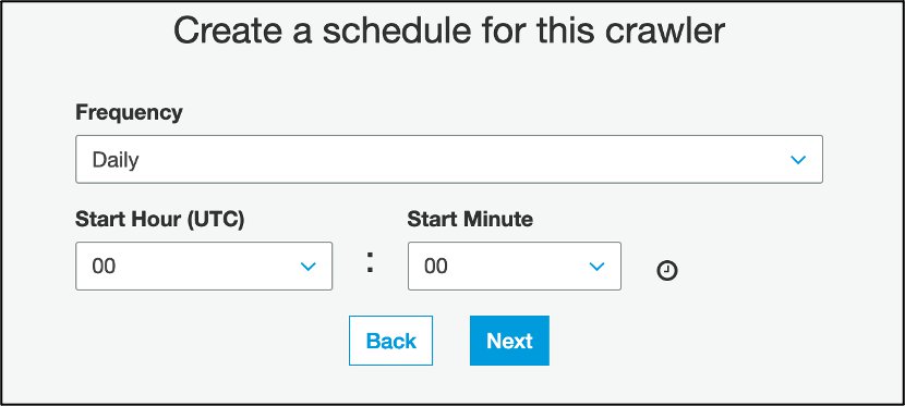
- In the Create a schedule for this crawler section, for Frequency, choose Daily.
You can also choose to run the crawler on demand.
- Enter your start hour and minute information.
- Choose Next.
- In the Configure the crawler’s output section, for Database, choose the database you created.
- Under Configuration options, select Ignore the change and don’t update the table in the data catalog.
- Select Update all new and existing partitions with metadata from the table.
- Choose Next.
- Review the settings and choose Finish.
For more information about configuring crawlers, see Crawler Properties.
When this crawler runs, it automatically creates an AWS Glue table.
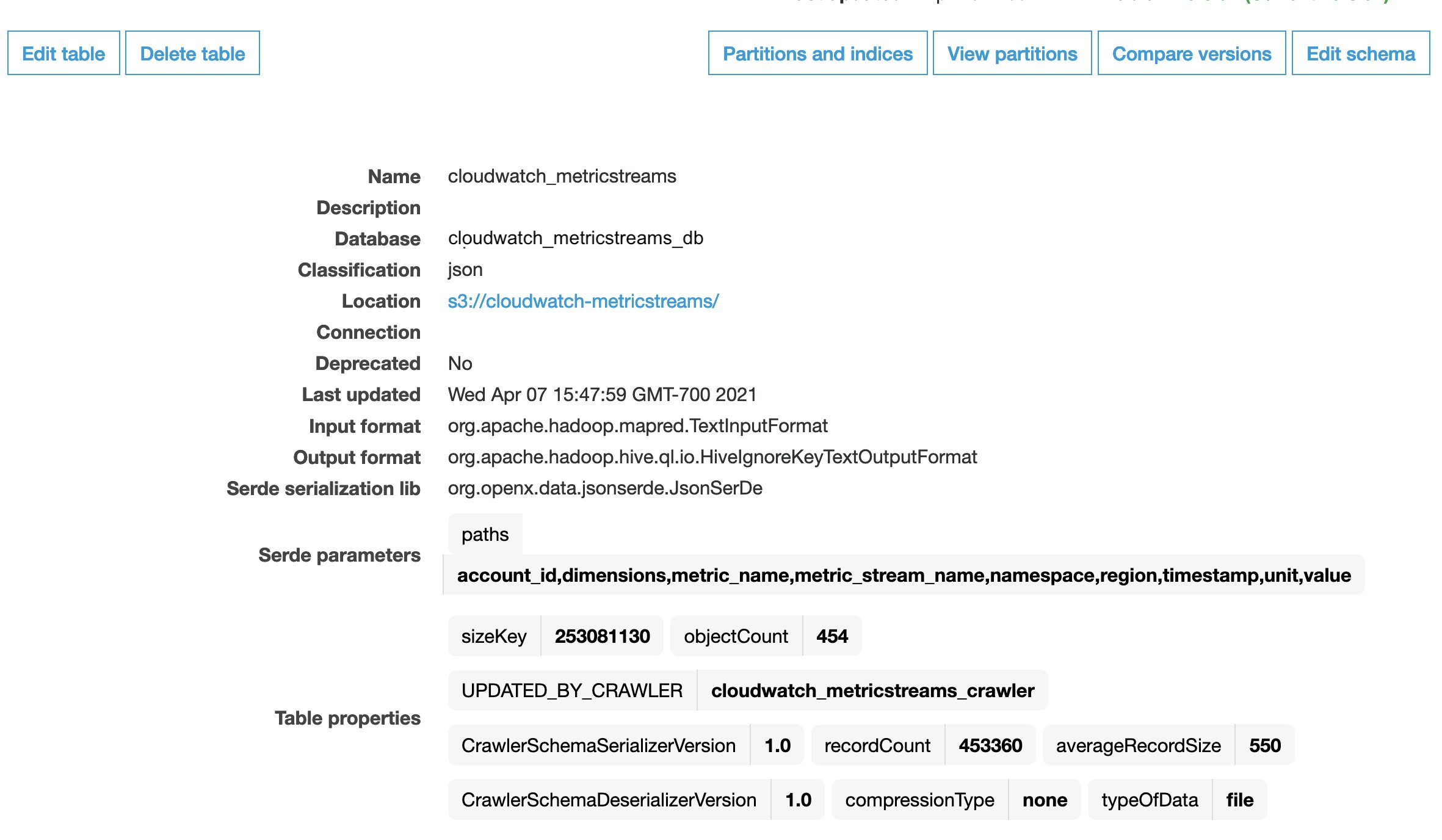
The crawler also creates the table schema and partitions based on the folder structure in the S3 bucket.
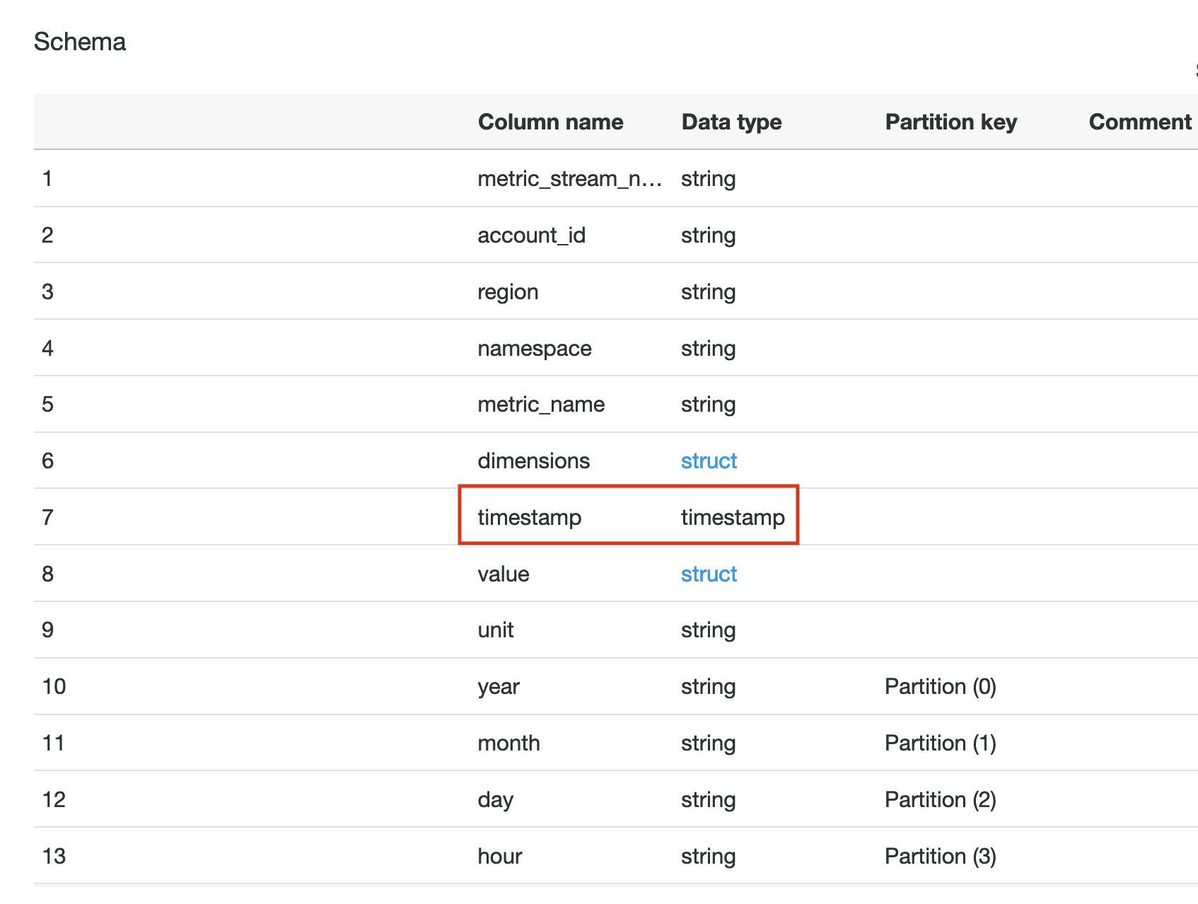
The timestamp column has the data type as bigint by default. We update the data type from biginit to timestamp to be able to write Athena queries more efficiently without any extra conversions on the fly.
- Choose Edit schema and update the
timestampcolumn data type totimestamp.
The schema now looks like the following screenshot.
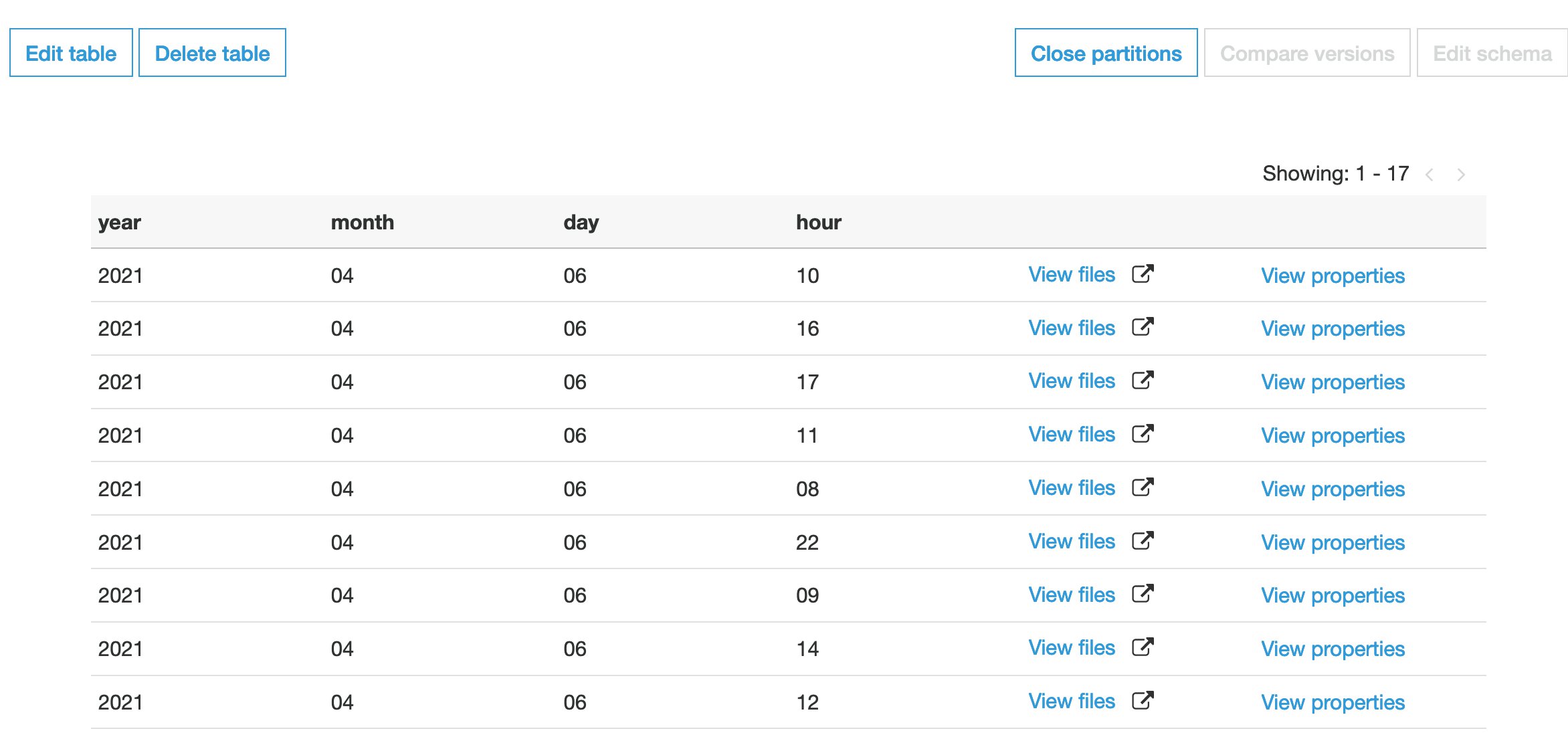
In this post, we configured the crawler to run daily. Every day at a specified time, it crawls new folders on your S3 bucket and creates partitions similar to those in the following screenshot.
Set up resources with AWS CloudFormation
If you want to set up all the AWS resources automatically, you can deploy an AWS CloudFormation template as follows:
- Sign in to the AWS Management Console with your IAM username and password.
- Choose Launch Stack.
![]()
- Choose Next.
- Enter the necessary parameters.
- Choose Next.
- Review the settings and choose Create stack.
Run Athena queries to identify database performance issues
Now that we have created a database and table using AWS Glue, we’re ready to analyze and find useful insights about our database services. We use Athena to run SQL queries to understand the usage of the database and identify underlying issues, if any. Athena is a serverless interactive query service that makes it easy to analyze data using standard SQL. You pay only for the queries that you run. With Athena, you don’t have to set up and manage any servers or data warehouses. You just point to your data in Amazon S3, define the schema, and start querying using the built-in editor.
In this section, we go through different scenarios for each service namespace.
Scenario 1: Compare year over year traffic increase impact
In this use case, our service receives more requests than usual on a specific day of the year, such as a big sporting event, new product launch event, or large retail day such as Prime Day. We want to compare year over year how the traffic increase impacted the efficiency of queries made to our DynamoDB table. This comparison allows us to make better decisions and strategies in setting the database configurations. Learning from past and present data can help us be aware of future traffic patterns and its impact on existing infrastructure.
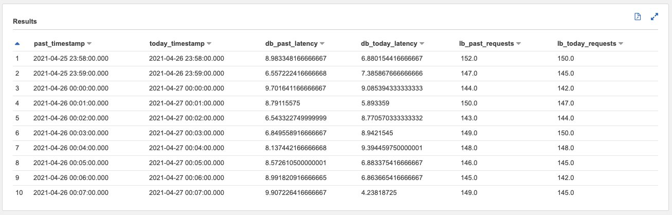
With the following example query, we can easily have a side-by-side comparison of web request count vs. DynamoDB latencies on BatchGetItem. When we analyze the metric SuccessfulRequestLatency, it’s a best practice to check the average latency. Occasional spikes in latency aren’t a cause for concern. However, if average latency is high, there might be an underlying issue that you need to resolve.
This query can also support day over day, week over week or year over year, by changing the DATE_ADD function and including all the relevant partitions in the WHERE clause.
The following screenshot shows our output.
Scenario 2: Identify any Amazon RDS database using over 80% of its maximum connections
DatabaseConnections is a very important metric that determines the number of database connections in use. Ideally, the number of current connections isn’t above 80% of your maximum connections. If the metric value is consistently at or more than 80%, you can consider moving to an RDS instance with higher RAM. For this post, let’s assume max_connections is 200. The following query works well even if you have thousands of database instances without running into any metric or search limitations:
Scenario 3: Identify if any EC2 instance is under- or over-provisioned
For this use case, we want to see if an EC2 instance is running at more than 80% or less that 5% of its CPU utilization.
CPUUtilization is one of the significant host-level metrics to monitor on an EC2 instance. If the metric value is consistently more than 80%, you may want to consider scaling it up. If it’s less than 5%, the instance may be over-provisioned, so consider scaling it down by switching it to a lower instance class. Let’s take an example where you have provisioned hundreds of instances before an event. You have load balancers in place to route traffic across these instances and you don’t want to use autoscaling for your business reasons. After the event, when you analyze the host metrics by using the following query, you can filter the over-utilized instances:
This can help you make better decisions for scaling your instances for the next event.
Scenario 4: Identify a DynamoDB table experiencing write or read request throttling
Throttling on DynamoDB metrics is a key indicator that one or more DynamoDB tables are under-provisioned for the amount of traffic they’re getting. Sudden traffic spikes can result in throttling. If the presence of the sparse metric ThrottledRequests is consistent across time, it’s a sign that the current provisioning settings should be revised, either manually or through DynamoDB autoscaling. We can use the following query to identify throttling:
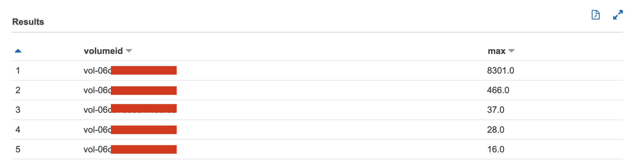
Scenario 5: Identify EBS volumes with a high number of read and write operations
VolumeReadOps and VolumeWriteOps metrics can help monitor the IOPS of your EBS volumes. These metrics provide the total number of read and write operations performed and can help identify if you have considered the most appropriate volume type. See the following code:
Clean up
Complete the following steps to clean up the AWS resources that we created as part of this post to avoid potential recurring charges.
- On the AWS CloudFormation console, choose the stack you used in this post.
- Choose Delete to delete the stack.
- On the Amazon S3 console, choose the bucket you used for this post.
- Choose Empty.
- Choose Delete.
Summary
In this blog, we discussed how to set up metric streams to continually stream CloudWatch metrics to a destination such as Amazon S3 with near-real-time delivery and retain it for as long as you wish. We then configured an AWS Glue database and crawler to automatically create a schema and partitions for your table. Furthermore, we used Athena to query CloudWatch metrics from multiple services like Amazon RDS, Amazon DynamoDB, Amazon EC2, and Amazon EBS to identify usage and performance issues from one single place.
You can extend this solution for your specific use case; this solution works well across many database types, scaling to thousands of instances, and supporting long-term metric retention. This provides a strong base for powerful analysis to get insights into your database performance and opportunities for ongoing improvement. You can tune your database configurations and make necessary modifications to improve your database performance.
Use this link to find more posts about monitoring databases with Amazon CloudWatch.
About the Author
 Mahek Pavagadhi is a Cloud Infrastructure Architect at AWS in San Francisco, CA. She has a master’s degree in Software Engineering with a major in Cloud Computing. She is passionate about cloud services and building solutions with it. Outside of work, she is an avid traveler who loves to explore local cafes.
 Gianluca Cacace is a Software Development Engineer at AWS in Dublin, Ireland. He has a master’s degree in Computer Engineering. He is passionate about scalability and design challenges on large-scale systems. In his spare time, he loves traveling and enjoys working on personal projects.