AWS Database Blog
Implement a correctness-safe Bloom filter lookup with Amazon ElastiCache for Valkey and Amazon Aurora PostgreSQL
High-throughput systems increasingly need to answer a membership question on every request: “Does this entity belong to a managed set?” They must do so under a hard latency budget and with zero tolerance for a false positive (wrongly reporting an item as present). Consider a payments platform processing thousands of transactions per second that must check whether a card is blocked for a specific merchant before authorizing. A false “yes” declines a legitimate transaction. A slow lookup causes timeouts at the point of sale.
A plain relational query is too slow for the hot path. A standalone Bloom filter is fast and memory-efficient, but it introduces false positives. This is unacceptable when a wrong match changes business outcomes. By composing a Bloom filter with an exact-match cache and a relational source of truth, you can serve most membership decisions in sub-millisecond time at P50, at peak throughput, while preserving correctness.
In a previous post, we covered how Bloom filters work in Amazon ElastiCache for Valkey, including scaling versus non-scaling filters, false-positive rate tuning, and over 90 percent memory savings compared to Set-based approaches. That post used the Bloom filter as the authoritative answer. This is acceptable when a false positive has no business impact.
In this post, we show you how to compose the Bloom filter into an end-to-end, correctness-safe, multi-tier lookup architecture. We walk through the three-tier design, composite key patterns for scoped membership queries, the consistency model that keeps all tiers in sync, and performance and cost considerations.
Solution overview
The pattern places three systems in sequence, each optimized for a different point on the latency-correctness spectrum:
- Tier 1 – Bloom filter (Amazon ElastiCache for Valkey) – A fast-negative gate. A single
BF.EXISTScall checks k hash positions in a compact bit array. If any bit is zero, the item is guaranteed absent and the request terminates immediately with no downstream I/O. If all bits are set, the item is possibly present and the request passes to Tier 2. - Tier 2 – Exact-match cache (ElastiCache for Valkey) – A deterministic lookup against a Valkey key that holds the confirmed membership record. A cache hit returns the authoritative answer in sub-millisecond time at P50 (about 1.8 ms at P99). A cache miss falls through to Tier 3.
- Tier 3 – Relational source of truth (Amazon Aurora PostgreSQL-Compatible Edition) – The canonical store. A point query by primary key returns the definitive answer, populates the cache on the read path, and drives all downstream tier updates.
The following diagram illustrates the request flow through the three tiers.
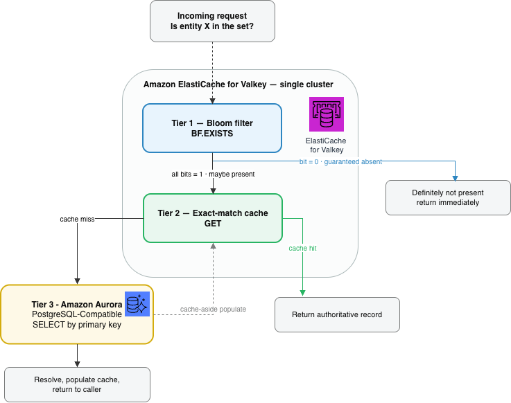
Figure 1: Correctness-safe three-tier membership lookup: the Bloom filter is a fast-negative gate, the exact-match cache serves confirmed hits, and Aurora PostgreSQL is the authoritative source of truth
Because ElastiCache for Valkey supports both Bloom filter commands (BF.EXISTS, BF.ADD) and standard key-value operations (GET, SET) on the same cluster, you can host Tier 1 and Tier 2 on a single ElastiCache cluster using distinct key prefixes. This reduces the architecture to two managed services: one ElastiCache cluster and one Aurora cluster.
What each tier guarantees
The pattern is correctness-safe because each tier makes a narrow, well-defined promise and the tiers are combined so that the source of truth always has the final word. It’s important to be precise about what each layer does and doesn’t guarantee.
- Bloom filter (Tier 1). Its error model is asymmetric with respect to its own contents. If
BF.EXISTSreturns 0, the key was never added to the filter, so there are no false negatives against the keys the filter has been told about. If it returns 1, the key is only possibly present. The chance that it’s a false positive is bounded by the false-positive rate (FPR), which you configure when you create the filter (a lower FPR costs more memory). The Bloom filter is an index of what has been propagated to it, not a source of truth about the database. - Exact-match cache (Tier 2). A hit returns a record that was authoritative when it was populated. Its freshness depends on the invalidation path and on a time-to-live (TTL), both described in the consistency model.
- Aurora (Tier 3). The database is the single source of truth. Every answer is ultimately confirmed against it, and it’s always authoritative.
A false positive from the Bloom filter is harmless: the request continues to the cache and, if needed, to Aurora, which resolves it correctly. The only cost is one extra lookup on a bounded fraction of requests (the FPR). This is the same lookup the request would have made without the Bloom filter.
The case that requires care is a false negative. A Bloom filter has no false negatives against its own contents, but the filter is a derived view that is updated after Aurora. In the window between an Aurora commit and its propagation to the filter, BF.EXISTS can return 0 for an item that already exists in the database. This is a functional false negative. Unhandled, this is the one way the pattern could return a wrong answer: in the payments example, authorizing a card that was just blocked. The consistency model closes this window with a mandatory recent-writes safety net and durable propagation, so the pattern is correctness-safe provided those mechanisms are in place. Because Aurora always has the final word, no failure produces a silently wrong positive. The worst case for a false positive is one extra database lookup.
Request flow in detail
The architecture creates a request funnel with four possible paths:
- Hot path (Bloom rejects) – The Bloom filter reports “definitely not present.” The request terminates in-memory with no cache or database I/O. This is the dominant path for workloads with high negative-query ratios such as ad deduplication, blocklist checks, and username availability, where 70–95 percent of lookups target items that don’t exist.
- Warm path (Bloom passes, cache hits) – All k bits are set. The request passes to the exact-match cache. The item is found and returned in sub-millisecond time at P50 (about 1.8 ms at P99).
- Cold path (Bloom passes, cache misses, database resolves) – A cache miss triggers a point query against Aurora PostgreSQL. The response populates the cache using the cache-aside pattern and returns to the caller.
- False-positive path (Bloom passes, item not found anywhere) – Identical to the cold path, except Aurora confirms the item doesn’t exist. At the 1 percent FPR used throughout this post, this happens on roughly 1 in 100 negative lookups. A stricter FPR makes it rarer at the cost of more memory.
Composite key design for scoped membership
A standard Bloom filter answers a binary question: “Is element X in the set?” Real-world systems often need scoped queries. “Is card X blocked for merchant Y?” or “Is user U restricted from channel C?” You can support these queries without creating a separate Bloom filter per scope by encoding both the entity and its qualifying attributes into a single composite key.
The pattern
Concatenate the entity ID with its scope and qualifying attributes into a single string before insertion. Use a tokenized ID rather than the raw value, so sensitive data never becomes a Valkey key (see the key design best practices). For example, derive a hash-based message authentication code (HMAC) of the card number under a managed key. In the examples that follow, 9f2b7c4a1d8e is such a token standing in for a card number, and MID_ANYCOMPANY is a merchant ID. The following example adds two scoped membership entries for the same card:
A scoped membership check then becomes a single BF.EXISTS call. The following example checks whether the card is blocked for debit transactions:
If the result is 0, the card is definitively not blocked for debit transactions. Serve the request immediately. If the result is 1, proceed to the cache and database for confirmation.
Bucketed composite keys
The filter stores one entry per (entity, scope) tuple, not one per entity. A single card blocked across several merchants and channels occupies several entries, so capacity is driven by the total tuple count (roughly entities × scopes per entity) plus headroom for churn, which can be several times the number of entities. For example, 100 million cards each blocked on a handful of merchants or channels can produce a few hundred million tuples. Size for tuples, not cards.
You don’t need a separate Bloom filter per entity. Instead, hash each composite key into a fixed number of buckets (for example, 200) and store it in that bucket’s filter. Bucket assignment must be deterministic and shared: both the live write path and the rebuild derive the Bloom key and its bucket from a single canonicalization-and-bucketing function. For example, bloom_key = "card:" + token + ":" + scope and bucket = hash(bloom_key) mod 200. If the two paths diverge in labels, delimiters, token derivation, hash function, or bucket count, they map the same logical membership to different buckets. A rebuilt filter then silently returns false negatives. Keep this function in one place and call it from both paths.
The following example reserves one bucket and adds a key. The 0.01 argument sets a 1 percent false-positive rate, the value used throughout this post. The FPR is a tunable trade-off between memory and the fraction of negative lookups that incur an extra check:
Because bucketing is hash-based, occupancy is uneven across buckets. The busiest bucket holds more than the average. Size each NONSCALING filter for the expected hottest-bucket occupancy, not the mean. A NONSCALING filter that exceeds its configured capacity degrades its false-positive rate. Alternatively, use scaling filters. In either case, monitor per-bucket occupancy with BF.CARD and BF.INFO so you can resize before the FPR drifts.
This approach yields 200 manageable Bloom filter objects rather than millions, while preserving the ability to query any entity-scope combination. Because each bucket is a distinct Valkey key, the buckets distribute across the shards of a Valkey (cluster mode) deployment, so the filter scales horizontally. Add shards to spread bucket memory and command throughput rather than growing a single object on one node.
Key design best practices
When designing composite keys, follow these recommendations:
- Use a consistent, self-describing key schema with a reserved delimiter, following Valkey key-naming conventions (for example,
card:{id}:merchant:{id}). Choose a delimiter that can’t appear in component values so key boundaries remain unambiguous. The labels add a small amount of memory overhead to the exact-match cache, but improve readability and operability. - Document the key schema across services so that producers and consumers agree on the encoding.
- Never use a raw card number (PAN) or other sensitive value as a key. Derive a stable token first, for example an HMAC of the ID under a managed key, so raw PANs never reach Valkey keys, cache values, the recent-writes set, or command logs. This is a Payment Card Industry Data Security Standard (PCI DSS) requirement.
The computational cost of composite keys is negligible. BF.EXISTS and BF.ADD have O(K) time complexity where K is the number of hash functions, independent of key length.
Consistency model
The database is always authoritative. The Bloom filter and the exact-match cache are derived views that are updated after the database, so they are eventually consistent with it. The goal is not to remove the gap between a database write and its propagation to the derived tiers, but to bound that gap and prevent it from ever producing an incorrect answer. The derived layers must never serve a stale “not present” for an item that exists, and the cache must not serve a changed record as confirmed.
Write-path ordering
Every write updates the database first, then the derived tiers:
- Write to Aurora PostgreSQL. The source of truth commits first.
- Invalidate the cache. Delete the corresponding Valkey key so the next reader repopulates it from the database.
- Update the Bloom filter. Add the new composite key with
BF.ADD.
Steps 2 and 3 run after the commit, so a partial failure leaves the derived tiers briefly out of sync with the database. Two windows can open:
- A missed
BF.ADD(step 3) leaves a new item absent from the Bloom filter. Tier 1 then returns “not present” and the request never reaches the database, which is a stale negative. This is the dangerous case (in the payments example, authorizing a card that was just blocked), and the recent-writes safety net described later is what closes it. - A missed cache invalidation (step 2) leaves an old record in Tier 2, so a reader receives a stale positive until the entry is corrected. A TTL on every Tier 2 entry bounds how long this can last.
To keep both windows short and self-healing, drive steps 2 and 3 from a durable, idempotent mechanism rather than best-effort calls. A transactional outbox, for example, retries the cache invalidation and the BF.ADD until each succeeds.
Because the cache is populated on read (the cache-aside pattern), it holds only values that were authoritative at population time. Serve the Tier 3 confirmation query from the writer, or another read-your-writes source. Otherwise the cache-aside path can reintroduce stale data. After step 2 invalidates a key, a concurrent miss that reads a pre-update row from a lagging replica would repopulate Tier 2 with the old value. Reading the confirmation path from the writer closes that race.
Handling deletions
Standard Bloom filters can’t remove elements, because clearing a bit could invalidate other keys that share the same hash positions. Valkey’s native Bloom filter is similarly add-only, with no delete command and no per-item count. Deletions are therefore handled outside the filter, with stale entries cleared during periodic rebuilds.
When an item is deleted, update Aurora and invalidate the exact-match cache immediately, so the authoritative tiers stop returning it right away. The Bloom filter might still report the deleted key as present until the next rebuild, but that is a bounded false positive. The request falls through to the cache and database, which no longer hold the record, at the cost of an extra cache or database check.
Scheduled rebuild – Query all active records from Aurora, build a fresh set of bucket filters in the background, and swap them in. RENAME is atomic for an individual key, so swapping roughly 200 buckets is a sequence of atomic renames with a brief window in which some buckets are new and others old. Correctness holds throughout: a stale positive falls through to the cache or database, and a bucket miss falls through to the cache, database, or recent-writes safety net. Run the export against an Aurora read replica to isolate the writer from scan load, and tune rebuild frequency to deletion volume.
Handling propagation lag
The failure mode to guard against is a functional false negative. An item exists in the database but has not yet propagated to the Bloom filter, for example a BF.ADD that is still being retried. Treat the “recent writes” set in Valkey as a required part of the write path rather than an optional extra. Add the entry to this set during step 1, before the write is acknowledged, so it’s visible to any reader that arrives during the propagation window. When the Bloom filter returns “not present,” check the recent-writes set before returning a negative. Size its TTL to exceed the worst-case propagation time. Include BF.ADD retries, change data capture (CDC) propagation, and any rebuild interval you rely on to land additions, so the window is never left uncovered. Because the set is consulted only on the minority path where the Bloom filter says “no,” it adds negligible overhead.
Aurora PostgreSQL as the source of truth
Amazon Aurora PostgreSQL-Compatible Edition is the authoritative store behind the derived tiers. This section covers the table schema that mirrors the composite key structure, connection pooling for high-concurrency access, and how to isolate Bloom filter rebuilds from production traffic.
Schema design
The membership table schema maps directly to the Bloom filter’s composite key structure. The following example creates a membership table with a composite primary key:
The composite primary key (entity_id, scope) supports single-row index lookups that complete in single-digit milliseconds, even with hundreds of millions of rows. The updated_at index supports incremental CDC queries for delta synchronization.
For time-scoped memberships, set each Tier 2 cache entry’s TTL to align with expires_at so the exact-match cache never returns an expired membership as a confirmed hit. The matching Bloom entry can linger until the next rebuild. That only raises the false-positive rate slightly, adding a few extra cache or database checks, and never affects correctness, because Aurora enforces expires_at and remains authoritative.
Connection pooling with Amazon RDS Proxy
For high-concurrency workloads, particularly serverless architectures with many short-lived connections, Amazon Relational Database Service (Amazon RDS) Proxy multiplexes client connections into a smaller pool of database connections using transaction-level reuse. This reduces the memory and CPU overhead that connection management places on the database, so Aurora can devote resources to serving queries rather than managing connections.
Bloom filter rebuild isolation
Full Bloom filter rebuilds scan millions of rows. Running these scans against the writer can degrade production query latency, so run the export against an Aurora read replica, which shares the same cluster storage volume as the writer.
A rebuild must reproduce exactly the keys the live write path would produce. Export the labeled key components, then let the rebuild worker apply the same canonicalization-and-bucketing function used at write time, so every key lands in the bucket it would live-write to:
The COPY command streams rows directly for a fast export. The rebuild worker then canonicalizes each row into its Bloom key and routes it to the correct bucket with the shared function before calling BF.ADD. It must not construct keys independently, or the rebuilt filter will diverge from the live one and return false negatives.
For very large sets, a multi-minute COPY against a live serving reader can still cause replication lag or standby query cancellation. Validate the scan under production load, use a dedicated reader, or source the rebuild from an Aurora export to Amazon Simple Storage Service (Amazon S3) rather than a serving instance.
Performance and cost considerations
This section examines the latency of each tier, how requests amplify across tiers, and how the pattern lowers database cost.
Latency by tier
The following table summarizes observed latency characteristics across the three tiers when the application and ElastiCache cluster are deployed in the same Availability Zone (AZ).
| Tier | Operation | P50 latency | P99 latency |
| Bloom filter | BF.EXISTS |
150-300 µs | ~1.8 ms |
| Exact-match cache | GET |
150-500 µs | ~1.8 ms |
| Aurora PostgreSQL | SELECT by PK |
1-5 ms | 5-15 ms |
The amplification factor
For a workload where 95 percent of lookups target items that don’t exist and the Bloom filter operates at a 1 percent FPR, the request distribution across tiers looks like the following:
| Tier | Traffic share | Explanation |
| Bloom filter | 100% | All requests enter here |
| Exact-match cache | ~5.95% | 5% true positives + 0.95% false positives from negative queries |
| Aurora PostgreSQL | <1% | Cache misses only |
The Bloom filter absorbs over 94 percent of all requests without any downstream I/O. The database handles less than 1 percent of total traffic, a reduction of approximately 99 percent in database load compared to querying Aurora for every request.
That reduction pays off in both latency and cost. Requests that the Bloom filter resolves finish in memory in the low hundreds of microseconds instead of paying a 1–5 ms Aurora point query (5–15 ms at P99). As a result, the overwhelming majority of requests are an order of magnitude faster on the hot path. It also changes how you provision the database. Because Aurora sees less than 1 percent of traffic rather than 100 percent, you can size the cluster (and any read replicas) for that residual load instead of peak request volume. This lowers instance and I/O cost. In effect, the in-memory tiers convert most of what would have been billable database work into far cheaper cache operations.
Conclusion
In this post, we showed how to compose a Bloom filter with an exact-match cache and a relational source of truth into a correctness-safe, multi-tier lookup architecture. The key design decisions are:
- Use the Bloom filter as an optimization, not an authority. False positives are bounded and harmless, and the database always has the final word.
- Encode scoped relationships into composite keys so that a single Bloom filter answers “Is X blocked for Y?” without per-scope filter proliferation.
- Keep tiers synchronized with periodic rebuilds, plus optional CDC for changes that reach the database outside the application write path, so additions propagate quickly while rebuilds clean up deletions.
- Host both Bloom and cache on a single ElastiCache cluster to minimize infrastructure and remove cross-cluster latency.
- Isolate rebuild queries on Aurora read replicas to protect writer performance.
With Bloom filters available as a first-class feature in ElastiCache version 8.1 for Valkey and later, this pattern requires no additional infrastructure or licensing. For workloads dominated by negative lookups such as ad deduplication, blocklist enforcement, fraud screening, and content filtering, the Bloom filter tier absorbs over 94 percent of traffic and reduces database load by approximately 99 percent. Typical (P50) response times stay below a millisecond, and P99 stays in the low single-digit milliseconds.
To get started, create an ElastiCache for Valkey 8.1 cluster, reserve your first Bloom filter with BF.RESERVE, and compose it with the cache-aside pattern you likely already have in place. For more information about Bloom filter commands and configuration, see Getting started with Bloom filters in the ElastiCache documentation.