AWS Big Data Blog
Accelerate Amazon DynamoDB data access in AWS Glue jobs using the new AWS Glue DynamoDB Export connector
Jan 2024: This post was reviewed and updated for accuracy.
Modern data architectures encourage the integration of data lakes, data warehouses, and purpose-built data stores, enabling unified governance and easy data movement. With a modern data architecture on AWS, you can store data in a data lake and use a ring of purpose-built data services around the lake, allowing you to make decisions with speed and agility.
To achieve a modern data architecture, AWS Glue is the key service that integrates data over a data lake, data warehouse, and purpose-built data stores. AWS Glue simplifies data movement like inside-out, outside-in, or around the perimeter. A powerful purpose-built data store is Amazon DynamoDB, which is widely used by hundreds of thousands of companies, including Amazon.com. It’s common to move data from DynamoDB to a data lake built on top of Amazon Simple Storage Service (Amazon S3). Many customers move data from DynamoDB to Amazon S3 using AWS Glue extract, transform, and load (ETL) jobs.

Today, we’re pleased to announce the general availability of a new AWS Glue DynamoDB export connector. It’s built on top of the DynamoDB table export feature. It’s a scalable and cost-efficient way to read large DynamoDB table data in AWS Glue ETL jobs. This post describes the benefit of this new export connector and its use cases.
The following are typical use cases to read from DynamoDB tables using AWS Glue ETL jobs:
- Move the data from DynamoDB tables to different data stores
- Integrate the data with other services and applications
- Retain historical snapshots for auditing
- Build an S3 data lake from the DynamoDB data and analyze the data from various services, such as Amazon Athena, Amazon Redshift, and Amazon SageMaker
The new AWS Glue DynamoDB export connector
The old version of the AWS Glue DynamoDB connector reads DynamoDB tables through the DynamoDB Scan API. Instead, the new AWS Glue DynamoDB export connector reads DynamoDB data from the snapshot, which is exported from DynamoDB tables. This approach has following benefits:
- It doesn’t consume read capacity units of the source DynamoDB tables
- The read performance is consistent for large DynamoDB tables
Especially for large DynamoDB tables more than 100 GB, this new connector is significantly faster than the traditional connector.
To use this new export connector, you need to enable point-in-time recovery (PITR) for the source DynamoDB table in advance.
How to use the new connector on AWS Glue Studio Visual Editor
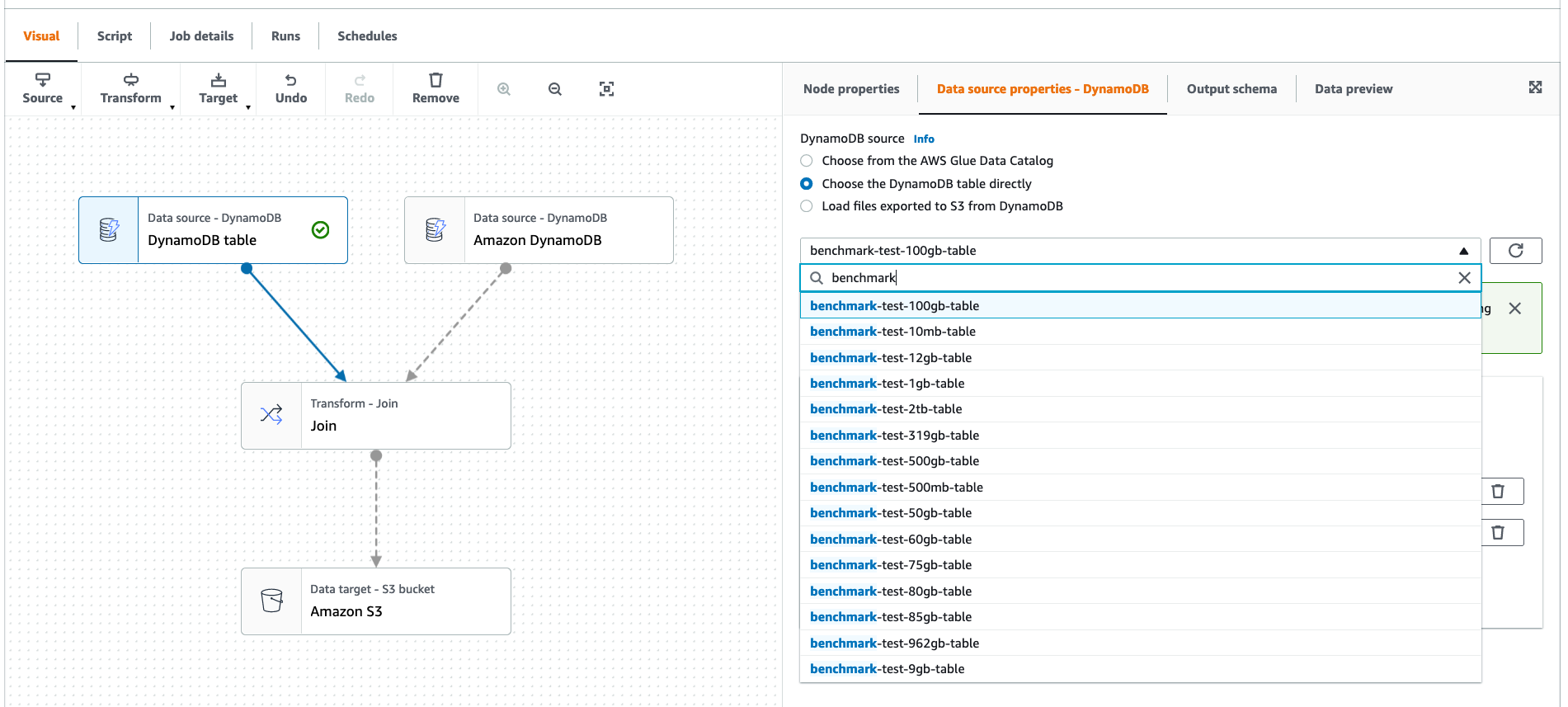
AWS Glue Studio Visual Editor is a graphical interface that makes it easy to create, run, and monitor AWS Glue ETL jobs in AWS Glue. The new DynamoDB export connector is available on AWS Glue Studio Visual Editor. You can choose Amazon DynamoDB as the source.

After you choose Create, you see the visual Directed Acyclic Graph (DAG). Here, you can choose your DynamoDB table that exists in this account or Region. This allows you to select DynamoDB tables (with PITR enabled) directly as a source in AWS Glue Studio. This provides a one-click export from any of your DynamoDB tables to Amazon S3. You can also easily add any data sources and targets or transformations to the DAG. For example, it allows you to join two different DynamoDB tables and export the result to Amazon S3, as shown in the following screenshot.
The following two connection options are automatically added. This location is used to store temporary data during the DynamoDB export phase. You can set S3 bucket lifecycle policies to expire temporary data.
- dynamodb.s3.bucket – The S3 bucket to store temporary data during DynamoDB export
- dynamodb.s3.prefix – The S3 prefix to store temporary data during DynamoDB export
How to use the new connector on the job script code
You can use the new export connector when you create an AWS Glue DynamicFrame in the job script code by configuring the following connection options:
- dynamodb.export – (Required) You need to set this to
ddbors3 - dynamodb.tableArn – (Required) Your source DynamoDB table ARN
- dynamodb.simplifyDDBJson – (Optional) If set to
true, performs a transformation to simplify the schema of the DynamoDB JSON structure that is present in exports. The default value isfalse. - dynamodb.s3.bucket – (Optional) The S3 bucket to store temporary data during DynamoDB export
- dynamodb.s3.prefix – (Optional) The S3 prefix to store temporary data during DynamoDB export
The following is the sample Python code to create a DynamicFrame using the new export connector:
The new export connector doesn’t require configurations related to AWS Glue job parallelism, unlike the old connector. Now you no longer need to change the configuration when you scale out the AWS Glue job. It also doesn’t require any configuration regarding DynamoDB table read/write capacity and its capacity mode (on demand or provisioned).
DynamoDB table schema handling
By default, the new export connector reads data in DynamoDB JSON structure that is present in exports. The following is an example schema of the frame which simulates customer review data:
To read DynamoDB item columns without handling nested data, you can set dynamodb.simplifyDDBJson to True. The following is an example of the schema of the same data where dynamodb.simplifyDDBJson is set to True:
Data freshness
Data freshness is the measure of staleness of the data from the live tables in the original source. In the new export connecor, the option dynamodb.export impacts data freshness.
When dynamodb.export is set to ddb, the AWS Glue job invokes a new export and then reads the export placed in an S3 bucket into DynamicFrame. It reads exports of the live table, so data can be fresh. On the other hand, when dynamodb.export is set to s3, the AWS Glue job skips invoking a new export and directly reads an export already placed in an S3 bucket. It reads exports of the past table, so data can be stale, but you can reduce overhead to trigger the exports.
The following table explains the data freshness and pros and cons of each option.
| .. | dynamodb.export Config | Data Freshness | Data Source | Pros | Cons |
|---|---|---|---|---|---|
| New export connector | s3 |
Stale | Export of the past table |
|
|
| New export connector | ddb |
Fresh | Export of the live table |
|
|
| Old connector | N/A | Most fresh | Scan of the live tables |
|
|
Performance
The following benchmark shows the performance improvements between the old version of the AWS Glue DynamoDB connector and the new export connector. The comparison uses the DynamoDB tables storing the TPC-DS benchmark dataset with different scales from 10 MB to 2 TB. The sample Spark job reads from the DynamoDB table and calculates the count of the items. All the Spark jobs are run on AWS Glue 3.0, G.2X, 60 workers.
The following chart compares AWS Glue job duration between the old connector and the new export connector. For small DynamoDB tables, the old connector is faster. For large tables more than 80 GB, the new export connector is faster. In other words, the DynamoDB export connector is recommended for jobs that take the old connector more than 5–10 minutes to run. Also, the chart shows that the duration of the new export connector increases slowly as data size increases, although the duration of the old connector increases rapidly as data size increases. This means that the new export connector is suitable especially for larger tables.

With AWS Glue Auto Scaling
AWS Glue Auto Scaling is a new feature to automatically resize computing resources for better performance at lower cost. You can take advantage of AWS Glue Auto Scaling with the new DynamoDB export connector.
As the following chart shows, with AWS Glue Auto Scaling, the duration of the new export connector is shorter than the old connector when the size of the source DynamoDB table is 100 GB or more. It shows a similar trend without AWS Glue Auto Scaling.

You get the cost benefits as only Spark driver is active for most of the time duration during the DynamoDB export (which is nearly 30% of the total job duration time with the old scan-based connector).
Conclusion
AWS Glue is a key service to integrate with multiple data stores. At AWS, we keep improving the performance and cost-efficiency of our services. In this post, we announced the availability of the new AWS Glue DynamoDB export connector. With this new connector, you can easily integrate your large data on DynamoDB tables with different data stores. It helps you read the large tables faster from AWS Glue jobs at lower cost.
The new AWS Glue DynamoDB export connector is now generally available in all supported Glue Regions. Let’s start using the new AWS Glue DynamoDB export connector today! We are looking forward to your feedback and stories on how you utilize the connector for your needs.
About the Authors
 Noritaka Sekiyama is a Principal Big Data Architect on the AWS Glue team. He is responsible for building software artifacts that help customers build data lakes on the cloud.
 Neil Gupta is a Software Development Engineer on the AWS Glue team. He enjoys tackling big data problems and learning more about distributed systems.
 Andrew Kim is a Software Development Engineer on the AWS Glue team. His passion is to build scalable and effective solutions to challenging problems and working with distributed systems.
 Savio Dsouza is a Software Development Manager on the AWS Glue team. His team works on distributed systems for efficiently managing data lakes on AWS and optimizing Apache Spark for performance and reliability.