Machine learning (ML) methods for the field of computational chemistry are growing at an accelerated rate. Easy access to open-source solvers (such as TensorFlow and Apache MXNet), toolkits (such as RDKit cheminformatics software), and open-scientific initiatives (such as DeepChem) makes it easy to use these frameworks in daily research. In the field of chemical informatics, many ensemble computational chemical workflows require the ability to consume a large number of compounds and profile various descriptor properties.
This blog post describes a two-stage workflow. In the first stage, take approximately 1100 candidate molecules and use AWS Batch to calculate various 2D molecular descriptors using a Dockerized RDKit image. The original dataset from MoleculeNet.ai – ESOLV includes the measured logSolubility (mol/L) for each compound. In the second stage use Amazon SageMaker, with Apache MXNet, to develop a linear regression prediction model, The ML model will perform a 70/30 split of training and validation sets with a RMSE=0.925 and a goodness of fit (Rˆ2) of 0.9 after 30 epochs.
In this blog post, you create the workflow to process the simplified molecular-input line-entry system (SMILES) input, which you then feed into Amazon SageMaker to create a model that predicts the logSolubility.
Overview
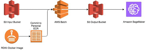
Start by storing the SMILES structures in an Amazon S3 bucket. Then build an Amazon Elastic Container Repository (Amazon ECR) image with a Python-based execution script and support libraries into a image and execute on AWS Batch. The output of the calculations is stored in another S3 bucket, which is input into Amazon Sagemaker.
Prerequisites
To follow the procedures in this blog post, you need an AWS account. You will create a Docker image on your local computer, so install and set up Docker. You also need to install the AWS command line interface (AWS CLI).
Stage 1: Using AWS Batch
AWS Batch is a managed service for running jobs from containerized applications stored in the Amazon ECR registry. An “amazonlinux:latest” image, which contains the base operating system (OS) for installing the tools needed to execute the workflow, was pulled from the public Docker registry. After you install Docker, open a command line shell and run the following command:
docker pull amazonlinux:latest
After pulling the image layers, start an interactive session to prepare the image for the descriptor calculations in AWS Batch. Install the AWS CLI, RDKit, and Boto3 framework packages in the image. In the running Docker container, run these commands:
docker run -it amazonlinux:latest
yum install epel-release aws-cli python-pip
pip install boto3
To install RDKit, first enable the repo. For code, see the EPEL 7 repository.
After enabling the repo, install it by running the following commands:
yum install python2-rdkit
mkdir -p /data
Add the following Python code to the image, then save it as /data/mp_calculate_descriptors.py.
from __future__ import print_function
import os
import sys
import boto3
import argparse
import uuid
import datetime
import subprocess
from rdkit import Chem
import multiprocessing as mp
from multiprocessing import Pool,Process
from rdkit.Chem import Descriptors as desc

# establish an Amazon S3 connection; an IAM role is needed to access Amazon S3
s3=boto3.client('s3')
# change to execution dir
os.chdir("/data")

# execute the main RDKit descriptor worker
def smiles_desc(smiles_str):
    output_desc=[]
    m = Chem.MolFromSmiles(smiles_str)
    output_desc=smiles_str, \
           desc.MolWt(m), \
           desc.Ipc(m), \
           desc.TPSA(m), \
           desc.LabuteASA(m), \
           desc.NumHDonors(m), \
           desc.NumHAcceptors(m), \
           desc.MolLogP(m), \
           desc.HeavyAtomCount(m), \
           desc.NumRotatableBonds(m), \
           desc.RingCount(m), \
           desc.NumValenceElectrons(m)

    desc_shard=str(output_desc).strip('()')
    smiles_out(desc_shard,csv_header)

    return
# write out the results to the local filesystem
def smiles_out(single_des_out,csv_header):
    fd=open("%s_smiles_result.csv" %csv_header,"a")
    fd.write(single_des_out)
    fd.write('\n')
    fd.close

# upload to an s3 bucket
def s3_upload(csv_header):
    env_S3_OUT=os.environ['OUTPUT_SMILES_S3']
    s3.upload_file("%s_smiles_result.csv" %csv_header,"%s" %env_S3_OUT,"%s_smiles_result.csv" %csv_header)

# calculate stat function
def calc_perf(input_file,timedelta):
    calc_perf_stat=int(len(input_file)/timedelta.total_seconds())
    return calc_perf_stat

if __name__ == "__main__":
# accepted args for command line execution
   parser = argparse.ArgumentParser(description='Process SMILES')
   parser.add_argument("-i", dest="smiles", required=False, help='SMILES string')
   parser.add_argument("-f", dest="smiles_file", required=False, help="File for Batch SMILES processing")
   args = parser.parse_args()

   smiles_str=args.smiles
   smiles_files=args.smiles_file
   csv_header=str(uuid.uuid4())

# if defined on the command line
   if smiles_str:
      print (smiles_desc(smiles_str))
      smiles_out(str(smiles_desc(smiles_str)),csv_header)
      s3_upload(csv_header)

# if importing a file
# by default, parallelism expands to available cores exposed to the container
   elif smiles_files:
      infile=open(smiles_files,"r")
      pool = mp.Pool()
      start_calc=datetime.datetime.now()
      smiles_list=list(infile)
      pool.map(smiles_desc,smiles_list)
      pool.close()
      end_calc=datetime.datetime.now()
      delta_calc=end_calc-start_calc
      stat_calc=calc_perf(smiles_list,delta_calc)
      print ("number of structures/sec: %s"%stat_calc)
      s3_upload(csv_header)

# if file is defined through env
# by default, parallelism expands to available cores exposed to the container
   elif os.getenv('INPUT_SMILES'):
      env_SMILES=os.environ['INPUT_SMILES']
      infile=open(env_SMILES,"r")
      pool = mp.Pool()
      start_calc=datetime.datetime.now()
      smiles_list=list(infile)
      pool.map(smiles_desc,smiles_list)
      pool.close()
      end_calc=datetime.datetime.now()
      delta_calc=end_calc-start_calc
      stat_calc=calc_perf(smiles_list,delta_calc)
      print ("number of structures/sec: %s"%stat_calc)
      s3_upload(csv_header)

# if file is in the S3 import bucket, specify an AWS BATCH job def
# by default, parallelism expands to available cores exposed to the container
   elif os.getenv('INPUT_SMILES_S3'):
      env_S3_SMILES=os.environ['INPUT_SMILES_S3']
      s3_dn=subprocess.Popen("aws s3 cp %s /data" %env_S3_SMILES, shell=True)
      s3_dn.communicate()
      s3_file=env_S3_SMILES.split('/')[-1]
      infile=open("/data/%s" %s3_file,"r")
      pool = mp.Pool()
      start_calc=datetime.datetime.now()
      smiles_list=list(infile)
      pool.map(smiles_desc,smiles_list)
      pool.close()
      end_calc=datetime.datetime.now()
      delta_calc=end_calc-start_calc
      stat_calc=calc_perf(smiles_list,delta_calc)
      print ("number of structures/sec: %s"%stat_calc)
      s3_upload(csv_header)

   else:
      print ("No SMILES FOUND...")
      sys.exit(0)
This code is the main engine for calculating the descriptors. The script reads the input SMILES file from the S3 bucket, calculates a series of descriptors, and then stores the results in another S3 bucket.
Open the Amazon S3 console and create buckets called rdkit-input-<initials> and rdkit-processed-<initials> with access limited to your AWS account.
Next, commit your Docker image to the Amazon ECR registry in your AWS account. Create a new registry by opening the Amazon ECS console, choosing Repositories on the left panel, and then Create repository. You get an endpoint similar to the following:
<account_number>.dkr.ecr.us-east-1.amazonaws.com/awsbatch/rdkit
To make the endpoint accessible to AWS Batch, push your Docker image to the endpoint:
# Get the temporary login credentials of your registry.
aws ecr get-login —no-include-email

# Execute the login command from "aws ecr get-login".
docker login <params>

# Commit the local container to a new docker image.
docker commit -m "setting up rdkit infra" <containerid> amazonlinux:rdkit

# Tag the new image with your Amazon ECR tag created in the Amazon ECS console.
docker tag amazonlinux:rdkit <account_number>.dkr.ecr.us-east-1.amazonaws.com/awsbatch/rdkit:latest

# Push the image to your private registery.
docker push <account_number>.dkr.ecr.us-east-1.amazonaws.com/awsbatch/rdkit:latest
AWS Batch requires that you set up a job with a job definition, which is then submitted to a job queue that is executed on a compute environment. The JSON job definition provides the input parameters for the RDKit job. The following is an example for this workflow:
{
    "jobDefinitionName": "rdkit1",
    "jobDefinitionArn": "arn:aws:batch:us-east-1:<account_number>:job-definition/rdkit1:1",
    "revision": 1,
    "status": "ACTIVE",
    "type": "container",
    "parameters": {},
    "retryStrategy": {
        "attempts": 1
    },
    "containerProperties": {
        "image": "<account_number>.dkr.ecr.us-east-1.amazonaws.com/awsbatch/rdkit:latest",
        "vcpus": 4,
        "memory": 2000,
        "command": [
            "python",
            "/data/mp_calculate_descriptors.py"
        ],
        "jobRoleArn": "arn:aws:iam::<account_number>:role/BatchS3Role",
        "volumes": [],
        "environment": [
            {
                "name": "OUTPUT_SMILES_S3",
                "value": "rdkit-processed-<initials>"
            },
            {
                "name": "INPUT_SMILES_S3",
                "value": "s3://rdkit-input-<initials>/deepchem.smiles"
            }
        ],
        "mountPoints": [],
        "ulimits": []
    }
}
In the job definition, define the OUTPUT_SMILES_S3 and INPUT_SMILES_S3 environmental variables. This is the path to the SMILES file uploaded to Amazon S3. This variable is passed into the Python script in the container. To ensure you have the correct permissions, define a jobRole (set in the IAM console) that has read and write access to Amazon S3. The Python script is natively parallelized, so the larger the instance, the greater the level of parallelization to process the SMILES file. The following table profiles the dataset using the c4 and m4 family of EC2 instances.
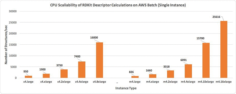
Run the AWS Batch job. You should see a file (*_smiles_result.csv) similar to the following in the rdkit-processed-<initials> bucket:

The original input file includes a column of measured logSolubility(mol/L). To prepare for the Amazon SageMaker stage that uses the SMILES as a primary key, append this column to the result file. This can be achieved by downloading the csv from S3 and uploading it again after appending the measured logSolubility values.
Stage 2: Using Amazon Sagemaker
In the Amazon SageMaker console, under Dashboard, choose Create notebook Instance, and then fill in the details of the interface as shown in the following screenshot. If this is your first time in the console, Amazon SageMaker will ask you to create an IAM role, which will need access to Amazon S3. It’s optional to set the VPC and subnet settings.
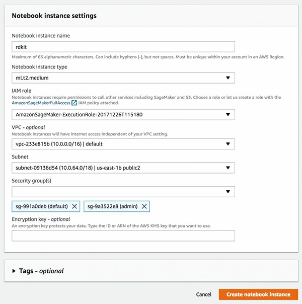
After you have completed these tasks choose Create notebook instance, It takes a few minutes for the instance to be created. After your instance is started choose Open, and you will be redirected to the instance and the Jupyter notebook interface.
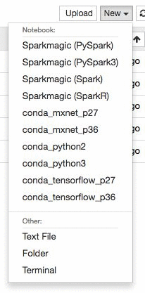
Create a new Jupyter notebook in the instance using the conda_mxnet_p27 environment. We also provide environments using TensorFlow as well as base Python 2 and Python 3 environments. Alternatively, you can simply download the entire notebook here.
Let’s create the notebook for training the candidate compounds. First, we need to define some S3 bucket variables in the location where we stored the result file from the first part of the workflow, after we have appended the solubility values.
#SET ENVIROMENT VARIABLE

#Set the bucket name for the processed bucket from AWS-Batch
#Set the key name for the output csv file from AWS-Batch

BUCKET_NAME="rdkit-processed-<initials>"
KEY_NAME="final_sol.csv"
Next we need to import the RDKit libraries into the environment:
#Install RDKit through conda
!conda install -y -c rdkit rdkit
Several dependencies will be installed. Next we will import the modules we will use in this exercise.
import os
import sys
import csv
import urllib
import boto
import subprocess
import numpy as np
import mxnet as mx
from rdkit import Chem
from rdkit.Chem import Draw
import multiprocessing as mp
import matplotlib.pyplot as plt
from ipywidgets import widgets
from IPython.html.widgets import *
from matplotlib.gridspec import GridSpec
from rdkit.Chem.Draw import IPythonConsole
from multiprocessing import Pool,Process
from rdkit.Chem import Descriptors as desc
Next we will read in the file from the deepchem GitHub.
# Download File
urllib.urlretrieve ("https://raw.githubusercontent.com/deepchem/deepchem/master/datasets/delaney-processed.csv", \
                    "delaney-processed.csv")
Now we will read in the SMILES from the file and parse the structures.
# Import File
infile=open("delaney-processed.csv","rb")
reader = csv.DictReader(infile)
smiles_list=list(reader)
m=[]
for i in range(len(smiles_list)):
    m.append(Chem.MolFromSmiles(smiles_list[i]['smiles']))
print "Number of Structures in file: %s" %len(m)
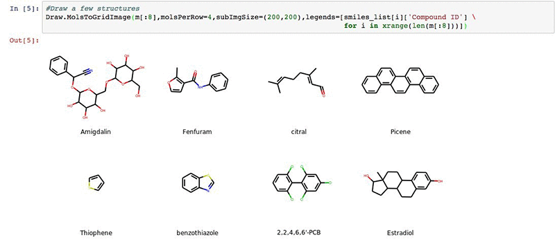
We can visualize a few of our structures in the deepchem set (optional).
#Draw a few structures
Draw.MolsToGridImage(m[:8],molsPerRow=4,subImgSize=(200,200),legends=[smiles_list[i]['Compound ID'] \
                                                                      for i in xrange(len(m[:8]))])
You will get an output:
Next we will import our results from the AWS Batch workflow described earlier.
# Import our result csv file from the AWS Batch workflow
conn=boto.connect_s3()
bucket=conn.get_bucket(BUCKET_NAME)
key=bucket.get_key(KEY_NAME)
key.get_contents_to_filename(KEY_NAME)

batch_file=open(KEY_NAME,"rb")
batch_reader = csv.reader(batch_file)
out_desc_all=list(batch_reader)
out_desc = [x[1:13] for x in out_desc_all]
We will split our data into a 70/30 training and validation sets with shuffling and prepare for modeling. The output will print out the data shapes for the training and validation sets.
# Define our input data arrays
out_desc_array=np.array(out_desc,dtype=np.float32)
np.random.shuffle(out_desc_array)
all_data = out_desc_array[:,0:11]
all_label = out_desc_array[:,11:12]
x_train,x_label, y_test,y_label = out_desc_array[:790,0:11], \
                                  out_desc_array[:790,11:12], \
                                  out_desc_array[790:,0:11], \
                                  out_desc_array[790:,11:12]

print np.shape(all_data)
print np.shape(all_label)
print np.shape(x_train)
print np.shape(x_label)
print np.shape(y_test)
print np.shape(y_label)
Now we define our linear modeling parameters. This is a relatively straightforward linear regression coupling batch normalization of the 2D descriptor set with a hyperbolic tangent activation. The output is a visual representation of the neural network.
# Define Model Parameters
import logging
logging.getLogger().setLevel(logging.DEBUG)

batch_size=20
train_iter = mx.io.NDArrayIter(x_train,x_label, batch_size, shuffle=True,label_name='lin_reg_label')
eval_iter = mx.io.NDArrayIter(y_test, y_label, batch_size, shuffle=False)
all_iter = mx.io.NDArrayIter(all_data, all_label, batch_size, shuffle=False)

train_iter.__dict__

X = mx.sym.Variable('data')
Y = mx.symbol.Variable('lin_reg_label')
fc1 = mx.symbol.BatchNorm_v1(data=X, name="BatchNorm_v1")
tanh1 = mx.symbol.Activation(fc1, act_type="tanh", name="tanh1")
fc2 = mx.sym.FullyConnected(data=tanh1, name='fc2', num_hidden = 1)
lro = mx.sym.LinearRegressionOutput(data=fc2, label=Y, name="lro")
shape={"data": (batch_size,790, 11)}
mx.viz.plot_network(lro,shape = shape)
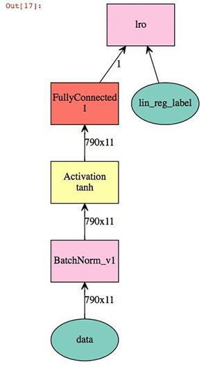
At this point we can train the model and check our validation score against the test.
# Train our model
model = mx.mod.Module(
    symbol = lro ,
    context = mx.cpu(),
    data_names=['data'],
    label_names = ['lin_reg_label']# network structure
)
model.bind(data_shapes=[train_iter.provide_data[0]], label_shapes=[train_iter.provide_label[0]])
model.init_params()
model.fit(train_iter, eval_iter,
            optimizer='sgd',
            optimizer_params={'learning_rate':0.01, 'momentum':0.9},
            num_epoch=50,
            eval_metric='rmse',
            batch_end_callback = mx.callback.Speedometer(batch_size, 10))
You should get the debug log of the training with an approximate speed of 20k samples/sec. Finally, we can plot our result score and use the model to predict the entire dataset.
# Plot our metrics - full cross validation
%matplotlib inline
from scipy import stats
all_preds=model.predict(all_iter).asnumpy()
eval_preds=model.predict(eval_iter).asnumpy()

plt.figure(figsize=(6,6), dpi=80)
plt.scatter(all_label,all_preds, label='All', c='blue',marker='.', alpha=0.2)
plt.scatter(y_label, eval_preds, label='Test/Evaluation', c='green',marker='.')
plt.xlim(-12,3)
plt.ylim(-10,2)
plt.title('Predicted vs Measured ESOLV DeepChem Set')
plt.xlabel('Measured logSolubility (mol/L)')
plt.ylabel('Predicted logSolubility (mol/L)')
plt.legend(loc=4)

print "pearson coefficient of all data: %s" %round(float(stats.pearsonr(all_label,all_preds)[0]),3)
print "pearson coefficient of evaluation data: %s" %round(float(stats.pearsonr(y_label,eval_preds)[0]),3)

delta_preds=all_preds-all_label
def plthist(x):
    fig = plt.figure(figsize=(6,6), dpi=80)
    plt.hist(delta_preds,bins=x,align='mid',range=(-4,4),rwidth=0.8)
    x=plt.xlabel('Element-wise Evaluation Prediction-Target')
interact(plthist,x=(2,50,1))
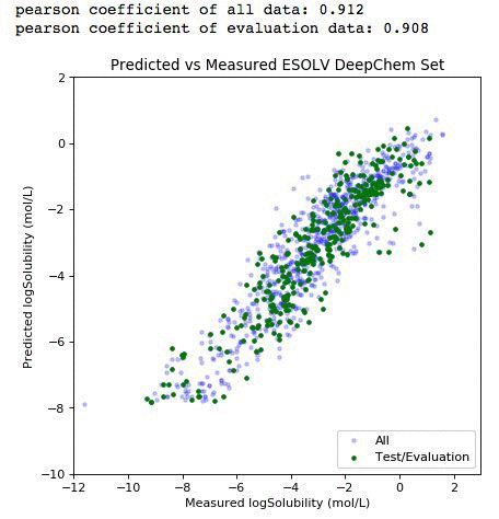
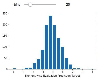
The light purple data points (left panel) comprise the entire dataset. The green subset is the compounds that have been selected for independent validation. The evaluation set adequately represents the diversity of the entire deepchem set with a validation score above 90 percent. The panel on the right represents the element-wise prediction error distribution. At this point, with the model built, you can create an endpoint and deploy it. You can follow along here for an example on how to deploy and create an endpoint for the model.
Summary
In this blog post you have successfully created a container-based RDKit platform in Amazon ECS and AWS Batch, processed a collection of compounds for molecular descriptor calculations, and developed an Apache MXNet ML model, through Amazon SageMaker, to predict the solubility.
I invite you to play around with the various model.fit() parameters in the Amazon SageMaker notebook. You can modify the optimizer, learning rates, and epochs. If you are able to improve the validation score please respond in the comments section of the blog.
If you have any questions, please leave them in the comments.
Next Steps
Connect with machine learning experts from across Amazon with the Amazon ML Solutions Lab.
About the Author
 Amr Ragab is a High Performance Computing Professional Services Consultant for AWS, devoted to helping customers run computational workloads at scale. In his spare time he likes traveling and finds ways to integrate technology into daily life.


 Amr Ragab is a High Performance Computing Professional Services Consultant for AWS, devoted to helping customers run computational workloads at scale. In his spare time he likes traveling and finds ways to integrate technology into daily life.