Artificial Intelligence
Enhanced performance for Amazon Bedrock Custom Model Import
You can now achieve significant performance improvements when using Amazon Bedrock Custom Model Import, with reduced end-to-end latency, faster time-to-first-token, and improved throughput through advanced PyTorch compilation and CUDA graph optimizations. With Amazon Bedrock Custom Model Import you can to bring your own foundation models to Amazon Bedrock for deployment and inference at scale.
These performance enhancements typically come with model initialization overhead that could impact container cold-start times. Amazon Bedrock addresses this with compilation artifact caching. This innovation delivers performance improvements while maintaining existing cold-start performance metrics that customers expect from CMI.
When deploying models with these optimizations, customers will experience a one-time initialization delay during the first model startup, but each subsequent model instance will spin up without this overhead—balancing performance with fast startup times during scaling.
In this post, we introduce how to use the improvements in Amazon Bedrock Custom Model Import.
How the optimization works
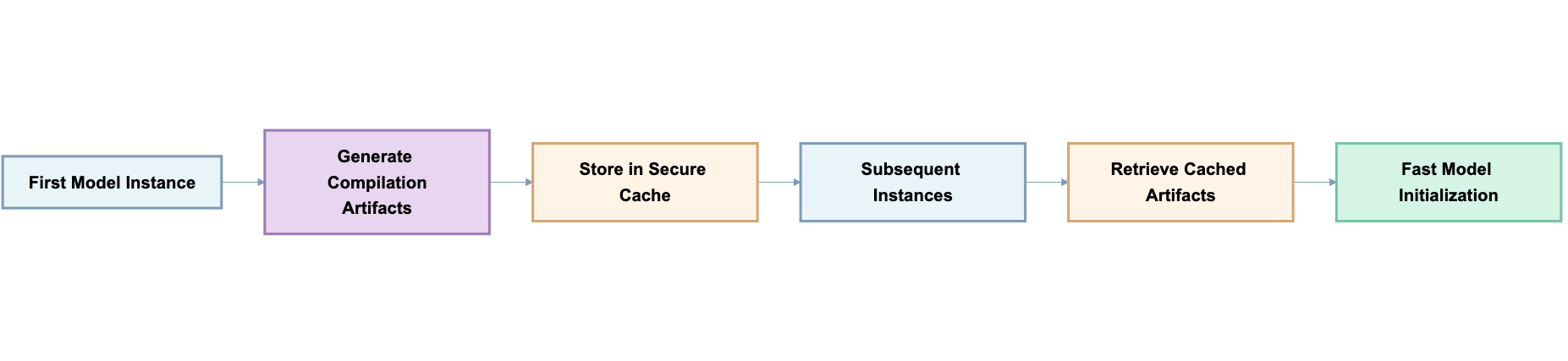
The inference engine caches compilation artifacts, removing repeated computational work at startup. When the first model instance starts, it generates compilation artifacts including optimized computational graphs and kernel configurations. These artifacts are stored and reused by later instances, so they skip the compilation process and start faster.
The system computes a unique identifier based on model configuration parameters such as batch size, context length, and hardware specifications. This identifier confirms cached artifacts match each model instance’s requirements, so they can be safely reused.
Stored artifacts include integrity verification to detect corruption during transfer or storage. If corruption occurs, the system clears the cache and regenerates artifacts. Models remain available during this process.
Performance improvements
We tested performance across different model sizes and workload patterns. The benchmarks compared models before and after the compilation caching optimizations, measuring key inference metrics under various concurrency levels from 1 to 32 concurrent requests.
Technical implementation: Compilation caching architecture
With a compilation caching architecture, performance improves because the system no longer repeats computational work at startup. When the first instance of a model starts, the inference engine performs several computationally intensive operations:
- Computational Graph Optimization: The engine analyzes the model’s neural network architecture and generates an optimized execution plan tailored to the target hardware. This includes operator fusion, memory layout optimization, and identifying opportunities for parallel execution.
- Kernel Compilation: GPU kernels are compiled and optimized for the specific model configuration, batch size, and sequence length. This compilation process generates highly optimized CUDA code that maximizes GPU utilization.
- Memory Planning: The engine determines optimal memory allocation strategies, including tensor placement and buffer reuse patterns that minimize memory fragmentation and data movement.
Previously, each new model instance repeated these operations independently, consuming significant initialization time. With compilation caching, the first instance generates these artifacts and helps store them securely. Subsequent instances retrieve and reuse these pre-compiled artifacts, bypassing the compilation phase entirely. The system uses a configuration-based identifier (incorporating model architecture, batch size, context length, and hardware specifications) to make sure cached artifacts match exactly with instance requirements, maintaining correctness while facilitating consistent optimized performance across the instances. The system includes checksum verification to detect corrupted cache files. If verification fails, the system automatically falls back to full compilation, facilitating reliability while maintaining the performance benefits when cache is available.
Benchmarking set up
We benchmarked under conditions that mirror production environments:
Test configuration: Each benchmark run deployed a single model copy per instance without auto-scaling enabled. This isolated configuration makes sure that performance measurements reflect the true capabilities of the optimization without interference from scaling behaviors or resource contention between multiple model copies. By maintaining this controlled environment, we can attribute performance improvements directly to the compilation caching enhancements rather than infrastructure scaling effects.
Workload patterns: We evaluated two representative I/O patterns that span common use cases:
- 1000/250 tokens (1000 input, 250 output): Represents medium-length prompts with moderate response lengths, typical of conversational AI applications, code completion tasks, and interactive Q&A systems
- 2000/500 tokens (2000 input, 500 output): Represents longer context windows with more substantial responses, common in document analysis, detailed code generation, and comprehensive content creation tasks
We chose these patterns because latency varies with the input-to-output ratio. across different token distributions, as latency characteristics can vary significantly based on the ratio of input processing to output generation.
Concurrency levels: Tests were conducted at six concurrency levels (1, 2, 4, 8, 16, 32 concurrent requests) to evaluate performance under varying load conditions. This progression follows powers of two, allowing us to observe how the system scales from single-user scenarios to moderate multi-user loads. The concurrency testing reveals whether optimizations maintain their benefits under increased load and helps identify the potential bottlenecks that emerge at higher request volumes.
Metrics: We captured comprehensive latency statistics across the test runs, including minimum, maximum, average, P50 (median), P95, and P99 percentile values. This complete statistical distribution provides insights into both typical performance and tail latency behavior. The charts in the following section show average latency, which gives a balanced view of overall performance. The full statistical breakdown is available in the accompanying data tables for readers interested in deeper analysis of latency distributions.
Performance metrics definitions
We measured the following performance metrics:
- Time to First Token (TTFT) – The time elapsed from when a request is submitted until the model generates and returns the first token of its response. This metric is critical for user experience in interactive applications, as it determines how quickly users see the model begin responding. Lower TTFT values create a more responsive feel, especially important for streaming applications where users are waiting for the response to begin.
- End-to-End Latency (E2E) – The total time from request submission to complete response delivery, encompassing the processing stages including input processing, token generation, and output delivery. This represents the full wait time for a complete response.
- Throughput – The total number of tokens (both input and output) processed per second across the concurrent requests. Higher throughput means you can serve more users with the same hardware.
- Output Tokens Per Second (OTPS) – The rate at which the model generates output tokens during the response generation phase. This metric specifically measures generation speed and is particularly relevant for streaming applications where users see tokens appearing in real-time. Higher OTPS values result in smoother, faster-appearing text generation, improving the perceived responsiveness of streaming responses.
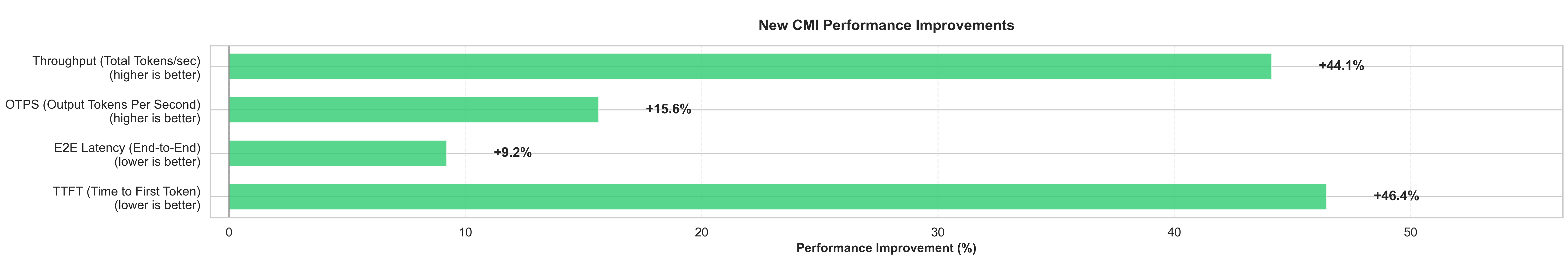
Inference performance gains
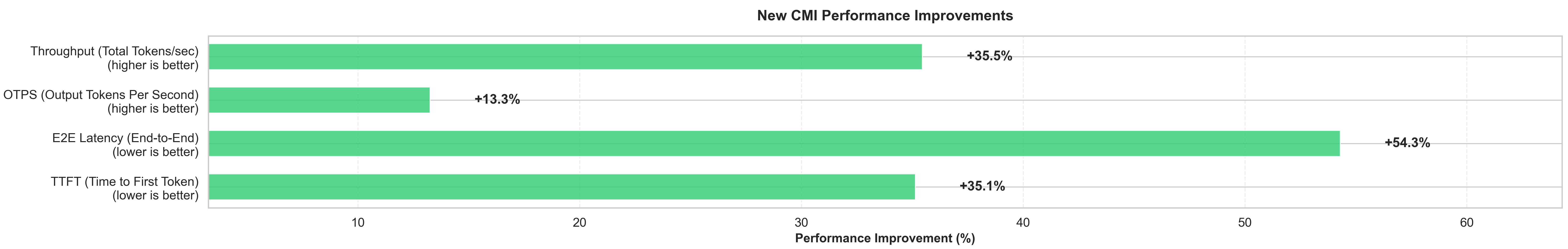
The compilation caching optimizations deliver substantial improvements across the measured metrics, fundamentally helping enhance the user experience and infrastructure efficiency. The following results showcase the performance gains achieved with two representative models, illustrating how the optimizations scale across different model architectures and use cases.
Granite 20B Code Model
As a larger model optimized for code generation tasks, the Granite 20B model demonstrates particularly impressive gains from compilation caching. The following P50 (median) metrics were measured using the 1000 input / 250 output token workload pattern:
- Time to First Token (TTFT): Reduced from 989.9ms to 120.9ms (87.8% improvement). Users see initial responses 8x faster.
- End-to-End Latency (E2E): Reduced from 12,829ms to 5,290ms (58.8% improvement). Complete requests finish in half the time for faster conversation turns.
- Throughput: Increased from 360.5 to 450.8 tokens/sec (25.0% increase). Each instance processes 25% more tokens per second.
- Output Tokens Per Second (OTPS): Increased from 44.8 to 48.3 tokens/sec (7.8% increase). Faster token generation improves streaming response quality.
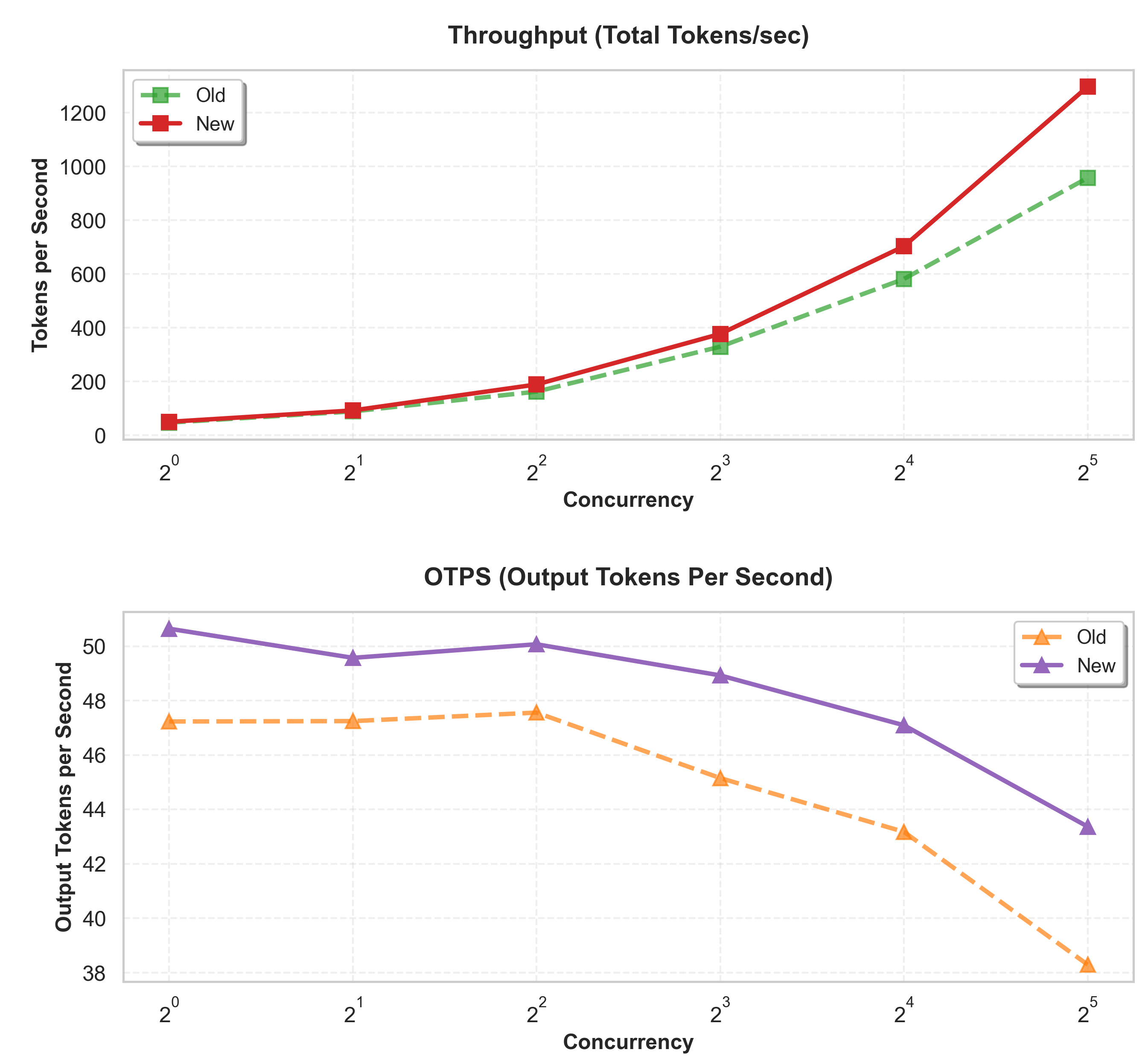
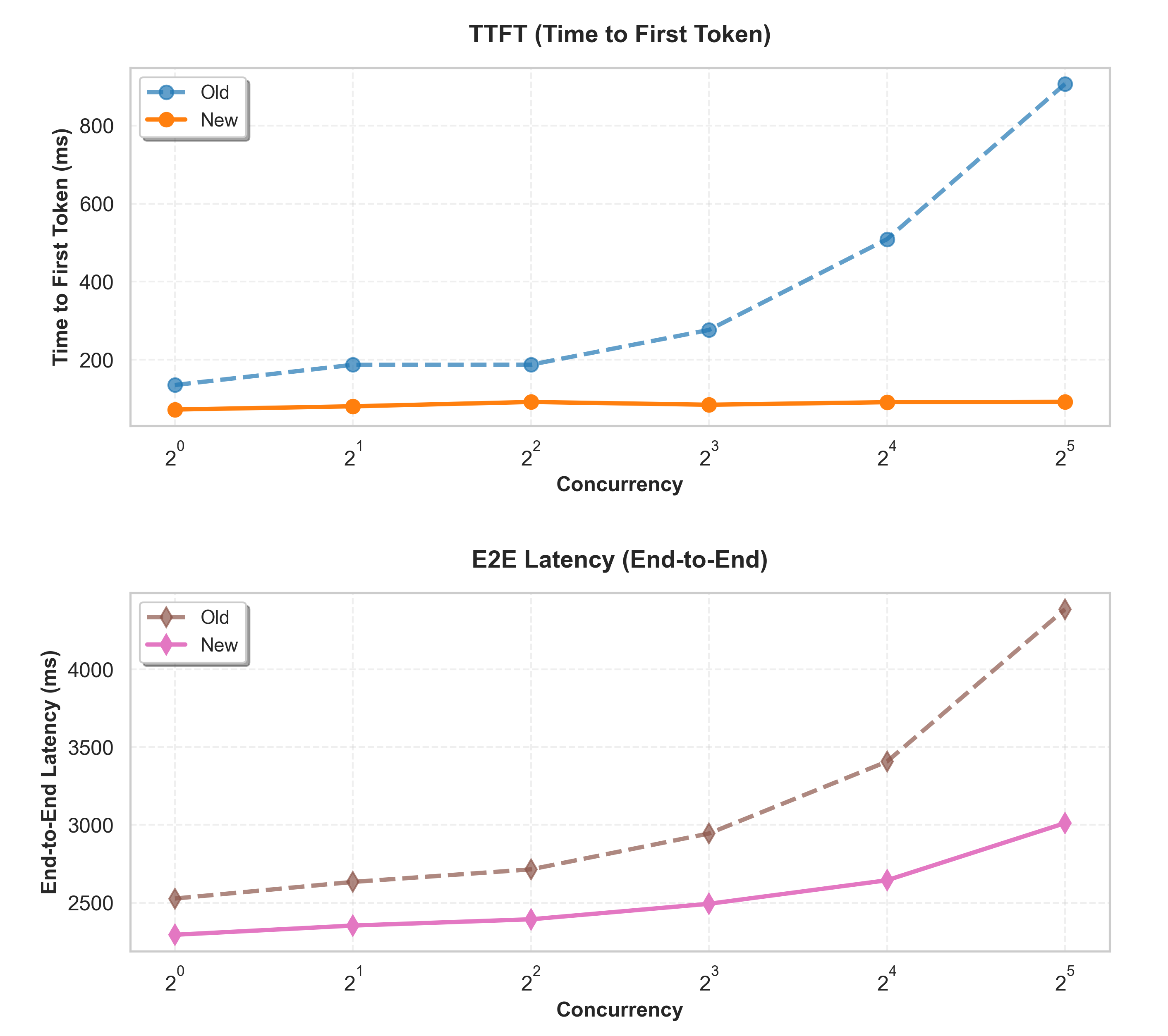
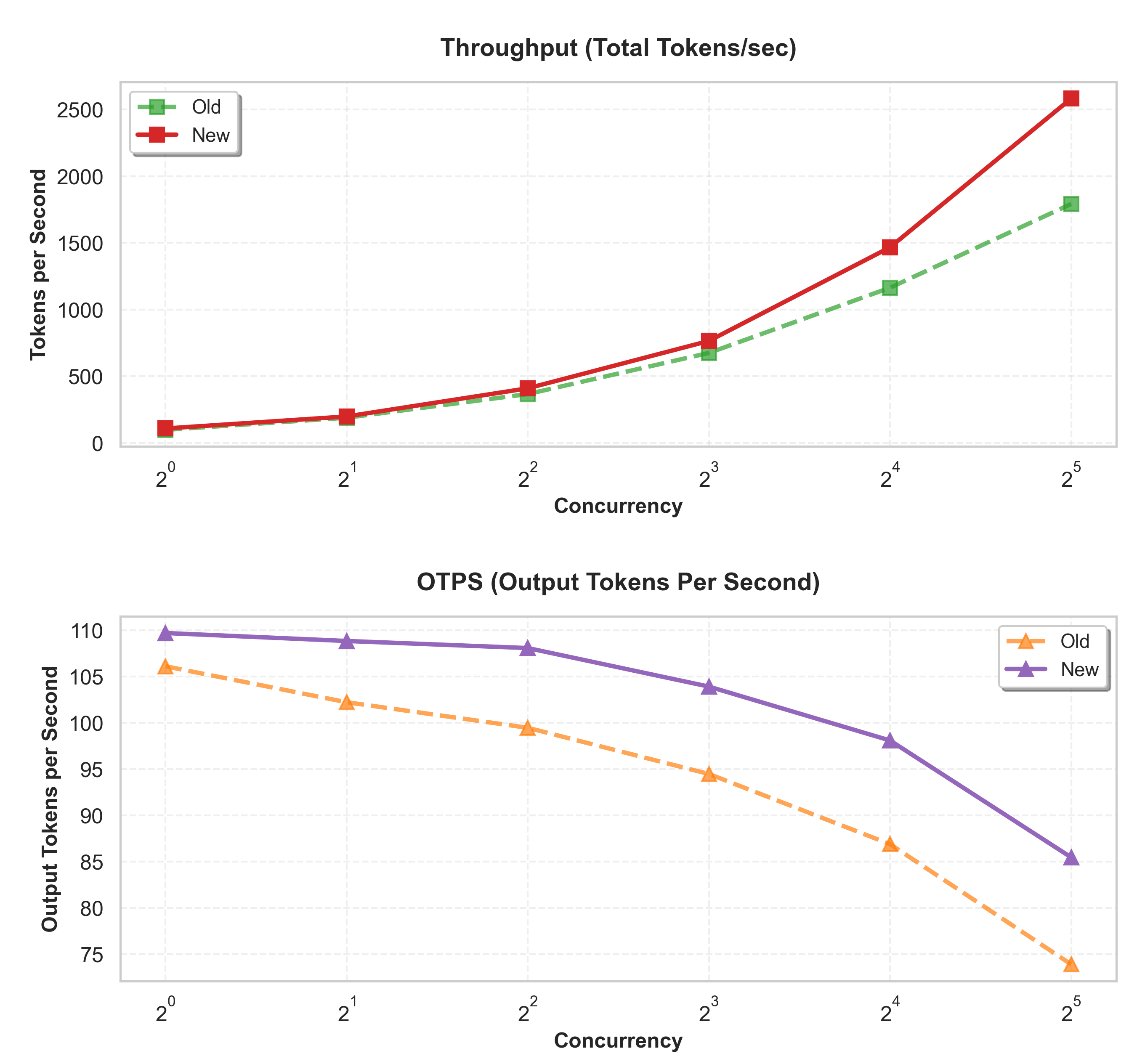
The following is a comparison of the metrics in the old and new containers for the granite-20b-code-base-8k model, using the average values in each case for an Input/Output pattern of 1000/250 tokens respectively. 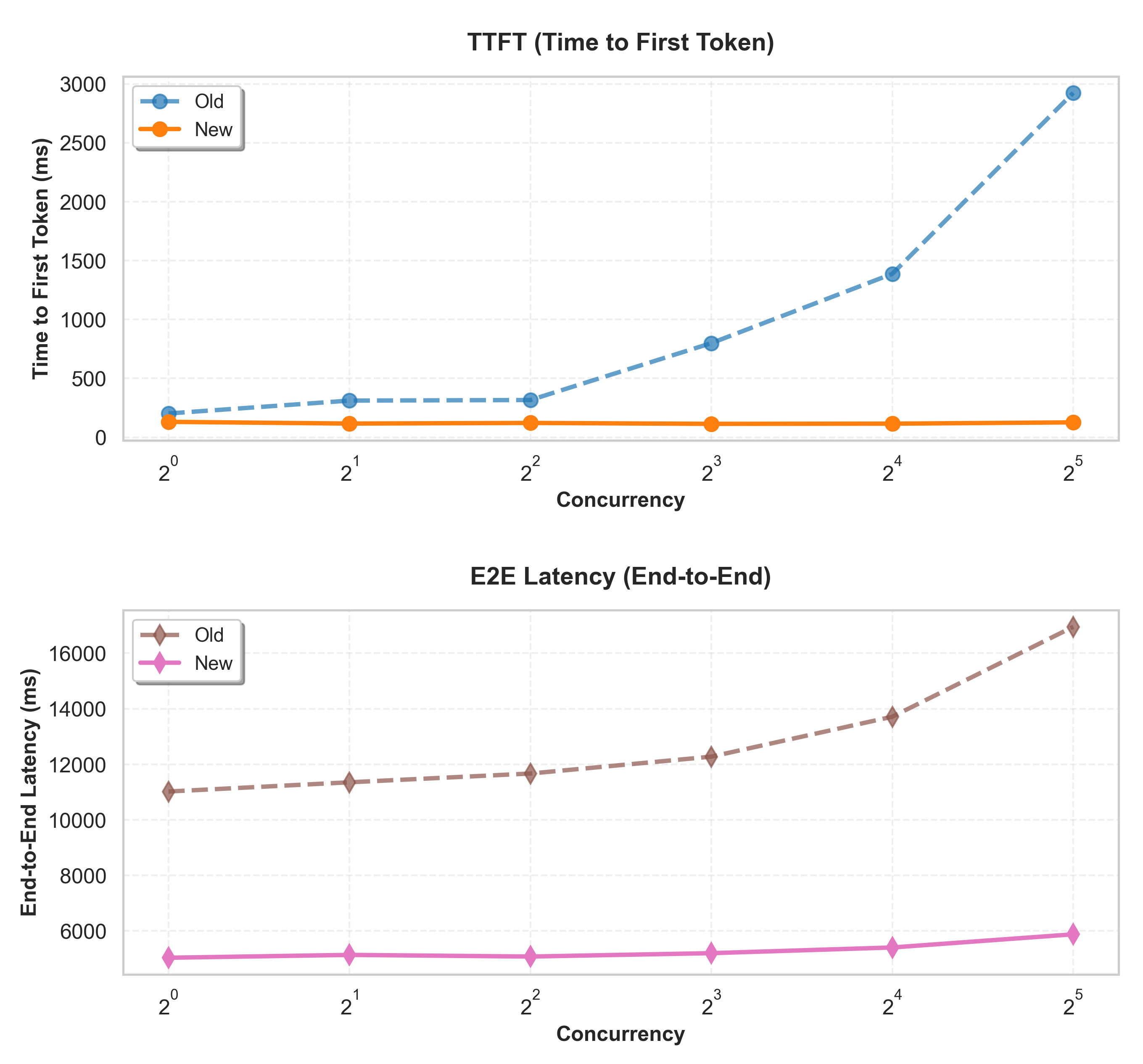
Llama 3.1 8B Instruct Model
The smaller Llama 3.1 8B model, designed for general instruction-following tasks, also shows significant performance improvements that demonstrate the broad applicability of compilation caching across different model architectures. The following P50 (median) metrics were measured using the 1000 input / 250 output token workload pattern:
- Time to First Token (TTFT): Reduced from 366.9ms to 85.5ms (76.7% improvement).
- End-to-End Latency: Reduced from 3,102ms to 2,532ms (18.4% improvement).
- Throughput: Increased from 714.3 tokens/sec to 922.0 tokens/sec (29.1% increase).
- Output Tokens Per Second (OTPS): Increased from 93.9 tokens/sec to 102.4 tokens/sec) (9.1% increase).
The following is a comparison of the metrics in the old and new containers for the llama3.1-8b model, using the average values in each case for an Input/Output pattern of 1000/250 tokens respectively.
The following table shows the full benchmarking metrics for Llama-3.1-8B-Instruct, single model copy, I/O tokens of 2000/500 respectively. Times are in milliseconds and RPS stands for requests per second.
| Container | Concurrency | TTFT_P50_sec | TTFT_P99_sec | E2E_P50_sec | E2E_P99_sec | OTPS_P50 | OTPS_P99 | Throughput_tokens_sec | RPS |
|---|---|---|---|---|---|---|---|---|---|
| Old | 1 | 113.54 | 253.24 | 4892.57 | 5015.59 | 105.67 | 41.99 | 101.81 | 0.2 |
| 2 | 112.41 | 288.53 | 5044.94 | 5242.21 | 102.05 | 41.14 | 196.02 | 0.39 | |
| 4 | 211.84 | 359.12 | 5263.9 | 5412.86 | 98.07 | 39.75 | 377.78 | 0.76 | |
| 8 | 319.95 | 509.61 | 5666.83 | 5905.78 | 93.87 | 38.63 | 701.95 | 1.4 | |
| 16 | 558.5 | 694.03 | 6424.99 | 6816.19 | 85.65 | 35.75 | 1235.08 | 2.47 | |
| 32 | 1032.31 | 1282.82 | 8055.76 | 8486.76 | 71.96 | 30.77 | 1967.64 | 3.94 | |
| New | 1 | 93.5 | 255.85 | 4550.11 | 4763.6 | 109.54 | 42.99 | 108.8 | 0.22 |
| 2 | 83.27 | 215.43 | 4670.78 | 4813.82 | 108.48 | 41.38 | 212.4 | 0.43 | |
| 4 | 82.05 | 207.42 | 4731.98 | 4848.53 | 107.91 | 43.76 | 419.6 | 0.84 | |
| 8 | 88.08 | 332.42 | 4938.4 | 5176.46 | 103.44 | 39.03 | 786.99 | 1.61 | |
| 16 | 89.75 | 287.81 | 5270.84 | 5449.96 | 96.31 | 43.92 | 1489.01 | 3.02 | |
| 32 | 105.04 | 242.07 | 6057.48 | 6212.99 | 84.62 | 16.2 | 2557.93 | 5.2 | |
| % Improvement | 1 | -17.65 | 1.03 | -7 | -5.02 | 3.66 | 2.37 | 6.87 | 6.93 |
| 2 | -25.93 | -25.34 | -7.42 | -8.17 | 6.3 | 0.59 | 8.36 | 8.47 | |
| 4 | -61.27 | -42.24 | -10.1 | -10.43 | 10.04 | 10.1 | 11.07 | 10.88 | |
| 8 | -72.47 | -34.77 | -12.85 | -12.35 | 10.2 | 1.04 | 12.11 | 14.47 | |
| 16 | -83.93 | -58.53 | -17.96 | -20.04 | 12.45 | 22.83 | 20.56 | 22.1 | |
| 32 | -89.82 | -81.13 | -24.81 | -26.79 | 17.59 | -47.37 | 30 | 31.93 |
The following table shows the full benchmarking metrics for Llama-3.1-8B-Instruct, single model copy, I/O tokens of 1000/250 respectively. Times are in milliseconds and RPS stands for requests per second.
The following table shows the full benchmarking metrics for granite-20B-code-base-8K, single model copy, I/O tokens of 2000/500 respectively. Times are in milliseconds and RPS stands for requests per second.
| Container | Concurrency | TTFT_P50_sec | TTFT_P99_sec | E2E_P50_sec | E2E_P99_sec | OTPS_P50 | OTPS_P99 | Throughput_tokens_sec | RPS |
|---|---|---|---|---|---|---|---|---|---|
| Old | 1 | 135.27 | 213.6 | 2526.95 | 2591.58 | 106.12 | 36.84 | 98.43 | 0.39 |
| 2 | 187.01 | 307.35 | 2633.8 | 2795.73 | 102.24 | 37.81 | 189.18 | 0.76 | |
| 4 | 187.41 | 284.01 | 2714.32 | 2917.68 | 99.48 | 35.73 | 366.71 | 1.47 | |
| 8 | 276.33 | 430.2 | 2944.84 | 3080.28 | 94.49 | 36.38 | 674.93 | 2.7 | |
| 16 | 508.86 | 729.68 | 3406.78 | 3647.68 | 86.9 | 35.47 | 1164.12 | 4.66 | |
| 32 | 906.54 | 1129.19 | 4385.52 | 4777.26 | 73.92 | 26.92 | 1792.15 | 7.21 | |
| New | 1 | 72.45 | 188.21 | 2294.31 | 2442.67 | 109.72 | 41.38 | 108.46 | 0.43 |
| 2 | 80.74 | 207.28 | 2353.47 | 2525.61 | 108.86 | 43.97 | 198.58 | 0.84 | |
| 4 | 91.84 | 222.23 | 2393.76 | 2543.41 | 108.1 | 44.75 | 409.74 | 1.64 | |
| 8 | 84.72 | 215.28 | 2493.32 | 2644.12 | 103.93 | 41.34 | 765.04 | 3.14 | |
| 16 | 91.28 | 206.43 | 2644.35 | 2754.45 | 98.11 | 36.65 | 1467.22 | 5.95 | |
| 32 | 92.26 | 329.83 | 3011.46 | 3243.96 | 85.48 | 36.59 | 2582.78 | 10.4 | |
| % Improvement | 1 | -46.44 | -11.88 | -9.21 | -5.75 | 3.39 | 12.32 | 10.19 | 10.19 |
| 2 | -56.82 | -32.56 | -10.64 | -9.66 | 6.48 | 16.29 | 4.97 | 10.12 | |
| 4 | -51 | -21.75 | -11.81 | -12.83 | 8.66 | 25.26 | 11.73 | 11.73 | |
| 8 | -69.34 | -49.96 | -15.33 | -14.16 | 9.99 | 13.63 | 13.35 | 16.21 | |
| 16 | -82.06 | -71.71 | -22.38 | -24.49 | 12.89 | 3.31 | 26.04 | 27.78 | |
| 32 | -89.82 | -70.79 | -31.33 | -32.1 | 15.64 | 35.95 | 44.12 | 44.11 |
The following table shows the full benchmarking metrics for Llama-3.1-8B-Instruct, single model copy, I/O tokens of 1000/250 respectively. Times are in milliseconds and RPS stands for requests per second.
| Container | Concurrency | TTFT_P50_sec | TTFT_P99_sec | E2E_P50_sec | E2E_P99_sec | OTPS_P50 | OTPS_P99 | Throughput_tokens_sec | RPS |
| Old | 1 | 258.19 | 294.23 | 11085.06 | 11264.87 | 47.12 | 26.02 | 46.11 | 0.09 |
| 2 | 312.07 | 602.62 | 11339.43 | 11628.22 | 46.41 | 24.51 | 88.36 | 0.18 | |
| 4 | 465.34 | 694.23 | 11600.97 | 11766.2 | 46.23 | 25.05 | 173.9 | 0.34 | |
| 8 | 836.29 | 1270.29 | 12387.4 | 12891.58 | 45.43 | 9.46 | 322.8 | 0.64 | |
| 16 | 1480.41 | 1879.95 | 13732.05 | 13923.09 | 43.01 | 19.96 | 585.75 | 1.17 | |
| 32 | 2532.85 | 3513.06 | 17117.17 | 17674.92 | 37.85 | 9.57 | 949.86 | 1.87 | |
| New | 1 | 132.15 | 253.91 | 9951.79 | 10171.01 | 50.58 | 27.87 | 50.09 | 0.1 |
| 2 | 110.34 | 337.33 | 10124.09 | 10391.73 | 49.94 | 27.8 | 91.72 | 0.2 | |
| 4 | 118.09 | 227.23 | 10023.25 | 10119.27 | 50.33 | 28.02 | 189.9 | 0.42 | |
| 8 | 155.44 | 299.35 | 10286.87 | 10431.96 | 49.18 | 26.09 | 377.21 | 0.83 | |
| 16 | 151.86 | 722.09 | 10632.11 | 11183.4 | 47.64 | 24.09 | 704.44 | 1.51 | |
| 32 | 161.64 | 291.93 | 11633.81 | 11754.09 | 43.78 | 25.25 | 1289.45 | 2.8 | |
| % Improvement | 1 | -48.82 | -13.71 | -10.22 | -9.71 | 7.35 | 7.09 | 8.63 | 13.93 |
| 2 | -64.64 | -44.02 | -10.72 | -10.63 | 7.62 | 13.41 | 3.79 | 13.6 | |
| 4 | -74.62 | -67.27 | -13.6 | -14 | 8.87 | 11.85 | 9.2 | 21.68 | |
| 8 | -81.41 | -76.43 | -16.96 | -19.08 | 8.25 | 175.82 | 16.86 | 29.2 | |
| 16 | -89.74 | -61.59 | -22.57 | -19.68 | 10.78 | 20.73 | 20.26 | 29.73 | |
| 32 | -93.62 | -91.69 | -32.03 | -33.5 | 15.66 | 163.9 | 35.75 | 49.6 |
The following table shows the full benchmarking metrics for granite-20B-code-base-8K, single model copy, I/O tokens of 1000/250 respectively. Times are in milliseconds and RPS stands for requests per second.
| Container | Concurrency | TTFT_P50_sec | TTFT_P99_sec | E2E_P50_sec | E2E_P99_sec | OTPS_P50 | OTPS_P99 | Throughput_tokens_sec | RPS |
|---|---|---|---|---|---|---|---|---|---|
| Old | 1 | 202.02 | 501.28 | 11019.77 | 11236.29 | 47.23 | 27.81 | 46.32 | 0.09 |
| 2 | 311.32 | 430.68 | 11351.65 | 11446.29 | 47.25 | 9.15 | 88 | 0.18 | |
| 4 | 316.22 | 773.8 | 11667.41 | 11920.88 | 47.56 | 9.11 | 161.67 | 0.34 | |
| 8 | 799.08 | 1074.4 | 12274.93 | 12436.3 | 45.15 | 22.08 | 328.94 | 0.65 | |
| 16 | 1387.43 | 1919.39 | 13711.78 | 14158.22 | 43.17 | 17.91 | 580.98 | 1.17 | |
| 32 | 2923.09 | 3466.83 | 16948.35 | 17582.53 | 38.29 | 14.34 | 957.06 | 1.89 | |
| New | 1 | 131.05 | 469.14 | 5036.18 | 5392.59 | 50.64 | 26.87 | 49.3 | 0.21 |
| 2 | 116.53 | 266.52 | 5138.18 | 5289.51 | 49.57 | 27.64 | 91.67 | 0.39 | |
| 4 | 121.73 | 297.81 | 5079.28 | 5276.06 | 50.07 | 27.2 | 188.33 | 0.78 | |
| 8 | 114.02 | 296.05 | 5201.04 | 5331.99 | 48.93 | 25.8 | 376.41 | 1.53 | |
| 16 | 115.65 | 491.06 | 5405.52 | 5759.79 | 47.09 | 24.91 | 702.54 | 2.94 | |
| 32 | 126.58 | 372.97 | 5879.65 | 6109.53 | 43.37 | 23.5 | 1296.34 | 5.43 | |
| % Improvement | 1 | -35.13 | -6.41 | -54.3 | -52.01 | 7.22 | -3.41 | 6.43 | 129.21 |
| 2 | -62.57 | -38.12 | -54.74 | -53.79 | 4.92 | 202.08 | 4.17 | 119.45 | |
| 4 | -61.5 | -61.51 | -56.47 | -55.74 | 5.28 | 198.64 | 16.49 | 128.25 | |
| 8 | -85.73 | -72.44 | -57.63 | -57.13 | 8.36 | 16.83 | 14.43 | 134.13 | |
| 16 | -91.66 | -74.42 | -60.58 | -59.32 | 9.08 | 39.11 | 20.92 | 150.92 | |
| 32 | -95.67 | -89.24 | -65.31 | -65.25 | 13.25 | 63.92 | 35.45 | 186.81 |
Performance consistency across load conditions
These improvements remain consistent across different concurrency levels (1-32 concurrent requests), demonstrating the optimization’s effectiveness under varying load conditions. The reduced latency and increased throughput enable applications to serve more users with better response times while using the same infrastructure.
The benefits remain consistent during scaling events. When auto-scaling adds new instances to handle increased traffic, those instances leverage cached compilation artifacts to deliver the same optimized performance. This facilitates consistent inference performance across the instances, maintaining a high-quality user experience during traffic spikes.
Customer impact
These optimizations improve performance during initial deployment, scaling, and instance replacement. The compilation artifact caching makes sure that the performance benefits remain consistent as new instances are added, without requiring each instance to repeat the compilation process.
Chatbots and AI content generators can add capacity faster during peak usage, reducing wait times. Development teams experience shorter deployment cycles when updating models or testing configurations.
Reduced Time to First Token makes applications feel more responsive. Higher Output Tokens Per Second means you can serve more users with existing infrastructure. You can handle larger workloads without adding proportional compute resources.
Faster instance initialization makes auto-scaling more predictable. You can maintain performance during traffic spikes without over-provisioning.
Conclusion
Amazon Bedrock Custom Model Import now delivers substantial improvements in inference performance through compilation artifact caching and advanced optimization techniques. These enhancements reduce time-to-first-token, end-to-end latency, and increase throughput without requiring customer intervention. The compilation artifact caching system makes sure that performance gains remain consistent as your application scales to meet demand.
Existing users can benefit immediately. New users can see enhanced performance from their first deployment. To experience these performance improvements, import your custom models to Amazon Bedrock Custom Model Import today. For implementation guidance and supported model architectures, refer to the Custom Model Import documentation.
About the authors
 Nick McCarthy is a Senior Generative AI Specialist Solutions Architect on the Amazon Bedrock team, focused on model customization. He has worked with AWS clients across a wide range of industries — including healthcare, finance, sports, telecommunications, and energy — helping them accelerate business outcomes through the use of AI and machine learning. Outside of work, Nick loves traveling, exploring new cuisines, and reading about science and technology. He holds a Bachelor’s degree in Physics and a Master’s degree in Machine Learning.
 Prashant Patel is a Senior Software Development Engineer in AWS Bedrock. He’s passionate about scaling large language models for enterprise applications. Prior to joining AWS, he worked at IBM on productionizing large-scale AI/ML workloads on Kubernetes. Prashant has a master’s degree from NYU Tandon School of Engineering. While not at work, he enjoys traveling and playing with his dogs.
 Yashowardhan Shinde is a Software Development Engineer passionate about solving complex engineering challenges in large language model (LLM) inference and training, with a focus on infrastructure and optimization. He has worked across industry and research settings, contributing to building scalable GenAI systems. Yashowardhan has a master’s degree in Machine Learning from the University of California, San Diego. Outside of work, he enjoys traveling, trying out new food, and playing soccer.
 Yanyan Zhang is a Senior Generative AI Data Scientist at Amazon Web Services, where she has been working on cutting-edge AI/ML technologies as a Generative AI Specialist, helping customers use generative AI to achieve their desired outcomes. Yanyan graduated from Texas A&M University with a PhD in Electrical Engineering. Outside of work, she loves traveling, working out, and exploring new things.