Artificial Intelligence
Train ALBERT for natural language processing with TensorFlow on Amazon SageMaker
At re:Invent 2019, AWS shared the fastest training times on the cloud for two popular machine learning (ML) models: BERT (natural language processing) and Mask-RCNN (object detection). To train BERT in 1 hour, we efficiently scaled out to 2,048 NVIDIA V100 GPUs by improving the underlying infrastructure, network, and ML framework. Today, we’re open-sourcing the optimized training code for ALBERT (A Lite BERT), a powerful BERT-based language model that achieves state-of-the-art performance on industry benchmarks while training 1.7 times faster and cheaper. This post demonstrates how to train a faster, smaller, higher-quality model called ALBERT on Amazon SageMaker, a fully managed service that makes it easy to build, train, tune, and deploy ML models.
Although this isn’t a new model, it’s the first efficient distributed GPU implementation for TensorFlow 2. You can use AWS training scripts to train ALBERT in Amazon SageMaker on p3dn and g4dn instances for both single-node and distributed training. The scripts use mixed-precision training and accelerated linear algebra to complete training in under 24 hours (five times faster than without these optimizations), which allows data scientists to iterate faster and bring their models to production sooner. It uses model architectures from the open-source Hugging Face transformers library. For more information, see the GitHub repo.
You can use natural language processing (NLP) models to improve search results, recommend relevant items, improve translation, and much more. In many use cases, you can use Amazon Comprehend, a fully-managed NLP service. The service identifies the language of the text; extracts key phrases, places, people, brands, or events; understands how positive or negative the text is; analyzes text using tokenization and parts of speech; and automatically organizes a collection of text files by topic. You can also use AutoML capabilities in Amazon Comprehend to build a custom set of entities or text classification models that are tailored uniquely to your organization’s needs.
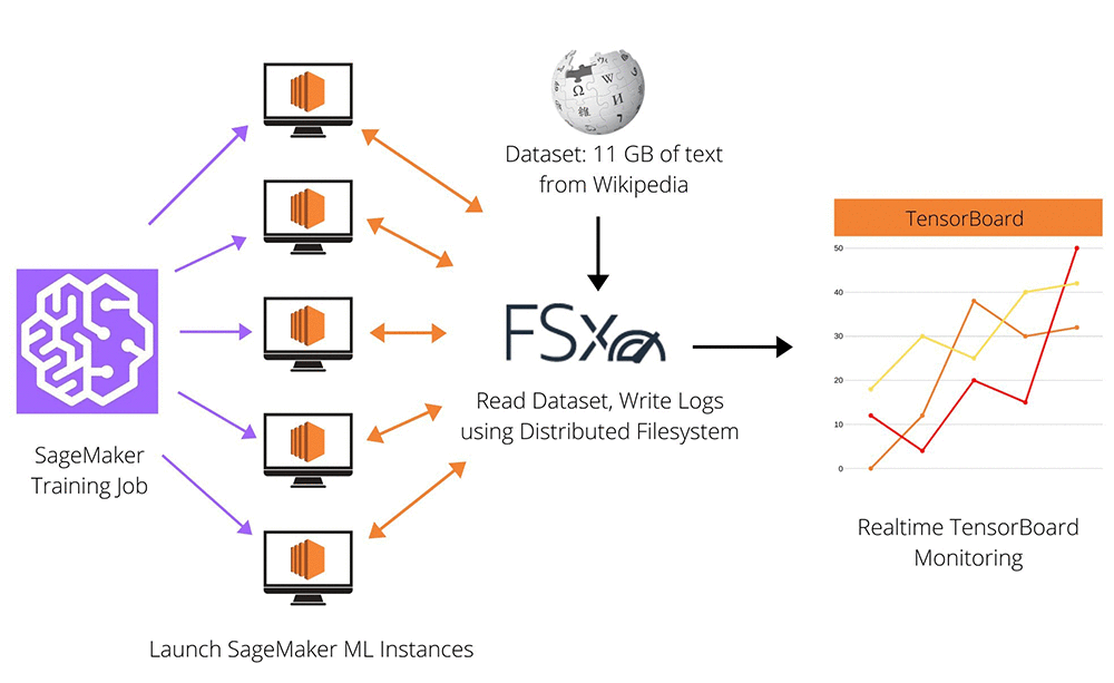
However, you may need to pretrain NLP models from scratch for your particular domain or language. Pretraining large language models often requires preparing 10-20 GB of raw text (the approximate size of English Wikipedia) and thousands of GPU-hours. It’s difficult to get the algorithms correct and efficient, and NLP development can be challenging because of the long training time before evaluating model quality. The following diagram shows an overview of the training infrastructure.

The workflow includes the following steps:
- The dataset (text from Wikipedia articles) is prepared and downloaded onto an FSx volume.
- Amazon SageMaker launches a distributed training job on many ML instances, which all read the sharded dataset from FSx.
- The instances write model checkpoints and TensorBoard logs to FSx.
- TensorBoard reads from FSx to monitor training progress in real time.
Overview of the ALBERT Model
The BERT language model was released in late 2018. In late 2019, AWS achieved the fastest training time by scaling up to 256 p3dn.24xlarge nodes, which trained BERT in just 62 minutes (19% faster than the previous record). You can extend these optimizations to train ALBERT using far fewer resources – only eight nodes to train ALBERT in less than a day.
ALBERT was released in late 2019. It can be trained 1.7 times faster with 18 times fewer parameters than its equivalent BERT model, which achieves even better performance. The improvements are threefold:
- Cross-layer weight tying – Reduces the number of parameters because each layer shares the same weights.
- Embedding factorization– Decouples the size of the hidden state from the size of the language vocabulary.
- Self-supervised sentence order prediction loss – Makes training more sample-efficient.
The biggest advantage of ALBERT is its parameter efficiency, because you can fit much larger batches into memory for quick inference. Best of all, you can use ALBERT in any scenario you previously used BERT, because they share the same architecture and embedding format. For more information and full model details, see ALBERT: A Lite BERT for Self-Supervised Learning of Language Representations.
There are two phases to model training: pretraining and finetuning. Pretraining is computationally expensive (98-99% of the load) compared to finetuning.
Pretraining
In the pretraining phase, the model learns a fill-in-the-blank task, called masked language modeling. Given a sentence like the following, the task is to fill in the blanks with predicted words or phrases.
Michael Jeffrey Jordan (born February 17, 1963), also known by his initials MJ, is an ___ former professional basketball player and the ___ owner of the Charlotte Hornets of the ___ Basketball Association (NBA).
The answers are American, principal, and National. There is also a secondary task, called sentence order prediction, to take two consecutive sentences, switch the order of half of them, and predict which sequences were flipped. Most of the text for this task comes from English Wikipedia.
Finetuning
In the finetuning phase, the model can perform many different kinds of tasks. This post focuses on question-answering. The Stanford Question Answering Dataset (SQuAD) is a unique NLP challenge. Much like a reading comprehension test, the input is a context paragraph and question, and the output is a subsection of the context text. Here is a sample context sentence:
The Amazon represents over half of the planet’s remaining rainforests, and comprises the largest and most biodiverse tract of tropical rainforest in the world, with an estimated 390 billion individual trees divided into 16,000 species.
with the question:
What percentage does the Amazon represent in rainforests on the planet?
The correct answers are “The Amazon represents over half of the planet’s remaining rainforest” or “over half”.
Comparison
The pretrained model learns contextual representations, then transfer learning enables you to reuse pretrained models for different downstream tasks with finetuning. There are two approaches to language modeling:
- Finetuning only (simple) – This takes less than an hour. Skip the pretraining phase by downloading an existing pretrained model. The downside is that this method may be inaccurate if your data style is different than what the downloaded model was pretrained on.
- Pretraining from scratch (advanced) – This requires more expertise and creates a more accurate model. Gather your own text dataset and train from scratch on your custom data.
The scripts in this post enable both options.
Transformers open-source library
The model architectures come from the Hugging Face transformers library, a popular open-source project for NLP. Using Transformers allows us to easily swap models for quick comparisons. We will continue to add support for new models, and open-source our work for machine learning reproducibility. We have already contributed several important pull requests (PR) upstream to the library, such as:
- Added AlbertForPreTraining architectures for TensorFlow and PyTorch (#4057).
- Diagnosed an accuracy issue in the TFAlbert models and helped retrain (#2837).
- Fixed a broken dropout layer and fixed a layer with duplicated bias (#3928).
- Added support for placing layer normalization at beginning of transformer layer (pre-layer norm) to stabilize training (#3929).
Training optimizations
You can run a distributed training job on Amazon SageMaker without provisioning, configuring, or managing the training cluster. All frameworks and dependencies come pre-installed and tuned for performance. All in all, these training optimizations speed up training by 10-15 times faster than a basic script. Specifically, the scripts use:
- Mixed-precision training – 3x faster. We use 16-bit floats rather than 32 bits, which can decrease the model’s required memory by up to 50%. This makes the model train faster and with larger batch sizes. We also incorporate loss scaling techniques to improve numerical precision.
- Accelerated linear algebra (XLA) – 2x faster. You can decrease memory usage and increase training speed by fusing certain operations and kernels together.
- Autograph optimizations – 3x faster. You can decrease memory usage and increase training speed by intelligently compiling certain functions into a TensorFlow graph.
- Efficient data loading – Language models require massive datasets. ALBERT uses 16GB; that’s 11,000 books plus all of English Wikipedia. We use Amazon FSx for Lustre, a high-performance filesystem built specifically for ML workloads. Unlike other storage solutions, FSx can connect to hundreds of machines in parallel, letting you store the dataset in a single central location and efficiently shard it in realtime.
Results
We reach the target accuracy on both the base and large models, with far less training time than is typically required.
- We pretrain for 125,000 steps with a total batch size of 4,096 across 8 p3dn.24xlarge nodes for 20 hours.
- We finetune for 8,144 steps with a total batch size of 48 on a single p3.16xlarge node for 20 minutes.
Pretraining for an even longer time period improves accuracy further. Since the focus is on minimizing both time and cost, we achieve comparatively strong accuracy with just a fraction of that compute budget.
SQuAD scoring is done via two metrics: exact match and F1. Exact match measures whether the selected answer matched exactly, and F1 is a measure combining both precision and recall of each word in the predicted answer. Both of these metrics range between 0-100, and F1 is greater than or equal to exact match.
| Model Size | Training Time | F1/Exact Match |
| ALBERT-base | 20 hours | 78.4/75.2 |
| ALBERT-large | 59 hours | 79.1/75.6 |
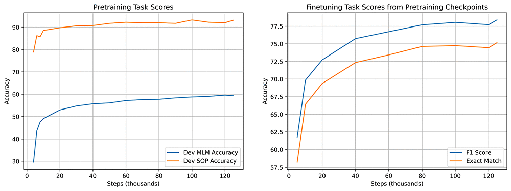
The following charts show model quality throughout training. The first shows scores on the masked language modeling (MLM) and sentence order prediction (SOP) tasks, which are used during pretraining. The second shows accuracy on question-answering (SQuAD) when finetuned from various checkpoints during pretraining. Improvements in the MLM and SOP tasks correlate with higher SQuAD accuracy.

Which instance type is the most time-efficient and cost-efficient for pretraining?
p3dn.24xlarge is fastest, while g4dn.12xlarge is the most cost-efficient. Language models require significant amounts of GPU memory. We have benchmarked three different GPU types against each other. More GPU VRAM means larger batch sizes and faster training steps at the expense of increased cost.
| Instance Type | Training Time | Nodes | Batch x Gradient Accumulation | Total Batch | Iterations/Second |
| ml.p3dn.24xlarge (8x32GB Tesla V100) | 20 hours | 8 | 32×2 | 4096 | 1.72 |
| ml.p3.16xlarge (8x16GB Tesla V100) | 39 hours | 8 | 16×4 | 4096 | 1.01 |
| ml.g4dn.12xlarge (4x16GB Tesla T4) | 78 hours | 16 | 16×4 | 4096 | 0.51 |
How efficiently do models scale from single-node to multi-node?
ALBERT has an incredible scaling efficiency of 95% when applying gradient accumulation. Scaling efficiency refers to the relative throughput of a model distributed across multiple nodes, as compared to a model on a single node. When training large language models on a limited number of nodes, gradient accumulation lets you use a large global batch size and attain the best accuracy. We also show that traditional scaling efficiency, measured in single-batch time, runs at 91% for the base model. ALBERT scales so well because the base model has 12 million parameters, compared with 110 million parameters for BERT. Its low communication overhead makes it an ideal candidate for distributed training. The following tables summarize scaling efficiency with and without gradient accumulation.
The following table shows scaling efficiency with gradient accumulation with sequences of 512 tokens:
| Model Size | 1-node sequences/second | 8-node sequences/second | Efficiency |
| ALBERT-base (batch 32, 2 acc) | 931 | 7045 | 95% |
| ALBERT-large (batch 16, 4 acc) | 322 | 2457 | 95% |
And this table shows scaling efficiency without gradient accumulation:
| Model Size | 1-node sequences/second | 8-node sequences/second | Efficiency |
| ALBERT-base (batch 32) | 888 | 6438 | 91% |
| ALBERT-large (batch 16) | 311 | 2109 | 85% |
Running the Model
Running the model includes the following steps:
- Create an FSx volume.
- Prepare data on FSx.
- Build a custom Docker container.
- Run a Horovod pretraining job on SageMaker.
- Run a Horovod finetuning job on SageMaker.
- Monitor training results on TensorBoard.
For complete instructions, see the aws-samples/deep-learning-models GitHub repository. The instructions below correspond with the v0.2 tag.
Creating an FSx volume
- In cloudformation/fsx.yaml, replace LustreBucketName with a unique S3 bucket name, and SubnetId with the main subnet of your default VPC.
- Enter the following command, which takes 5-10 minutes to complete.
- Go to the CloudFormation console, click on Stacks, and note the ID of your new FSx filesystem.
- In cloudformation/ec2.yaml, replace VPCId to match your VPC, specify KeyName as the name of an existing EC2 SSH key credential, set FileSystem to match the ID of the newly created FSx FileSystem, and set LustreBucketName to match the bucket specified in Step 1.
- Enter the following command, which takes 1-2 minutes to complete.
- You now have an FSx filesystem and an EC2 instance! SSH into the instance and run
ls /fsxto view your new mounted filesystem.
Preparing data on FSx
Prepare the dataset directly on the FSx filesystem by attaching and SSH-ing into an EC2 instance, no Amazon S3 upload required.
An easy way to get started is by downloading the Wikipedia dataset yourself, which contains a dump of 12GB text from English Wikipedia articles. Be sure to read and understand the dataset license before downloading, or use your own custom dataset. The data should be structured as a single text file, with one article per line. Then follow the instructions in the GitHub repository to preprocess the data.
Building a custom Docker container
To build and push your Docker container to Amazon Elastic Container Registry (ECR), run the following code:
Defining FSx environment variables
The launch scripts use environment variables to point to the FSx volume. Define the following variables on the command line:
Running a Horovod pretraining job on Amazon SageMaker
Run a horovod pretraining job on SageMaker with the following code:
Running a Horovod finetuning job on Amazon SageMaker
Your model name will be found in the Tensorboard logs or stdout logs from the pretraining script. Run a finetuning job with the following code:
Monitoring TensorBoard
- On your EC2 instance mounted on FSx, run the following code:
- On your local computer, run the following code:
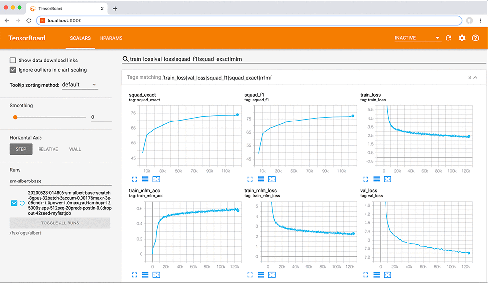
- Then open up localhost:6006 in your web browser to monitor the training! A sample run is shown below.

Conclusion
This post demonstrated how to train an ALBERT language model from scratch on Amazon SageMaker. Optimizations such as accelerated linear algebra and mixed-precision training can speed up training five times faster than the baseline. For more details and training scripts, visit the aws-samples/deep-learning-models GitHub repo.
About the Authors
 Jared Nielsen is a Machine Learning Engineer with AWS Deep Learning. He helps bring state-of-the-art machine learning research to customers. Outside of work, he enjoys rock climbing and reading great books.
 Derya Cavdar works as a software engineer at AWS Deep Learning. She obtained her PhD in computer engineering from Bogazici University in 2016. Her interests include deep learning, distributed systems and optimization.
 Aditya Bindal is a Senior Product Manager for AWS Deep Learning. He works on products that make it easier for customers to use deep learning engines. In his spare time, he enjoys playing tennis, reading historical fiction, and traveling.