AWS Storage Blog
Data discovery: How to find out what’s on your Amazon FSx for NetApp ONTAP volumes
Enterprise storage administrators manage hundreds of terabytes, and sometimes petabytes, of file data spanning business units, applications, and users. As that storage grows, so does the challenge of understanding what is actually stored in it. Administrators are asked to make capacity decisions, identify archive candidates, track storage costs, and support compliance reviews — but with no simple way to see the shape of their data, these questions are difficult and time-consuming to answer.
Amazon FSx for NetApp ONTAP provides fully managed, high-performance file storage in AWS with enterprise features such as fast backup and recovery, cross-region replication for disaster recovery, and TCO optimization driven by built-in compression and deduplication. With Amazon S3 Access Points for FSx for NetApp ONTAP, file data can be accessed via S3 APIs (as it were in an S3 bucket) in addition to NFS and SMB. This enables a new class of data management capabilities for FSx for NetApp ONTAP, including the ability to discover and understand file data using the same AWS analytics and AI services that customers already use for their object storage, without creating redundant copies or re-architecting their storage environment.
In this post, we describe a solution that gives administrators a continuously refreshed, SQL-queryable catalog of their FSx for NetApp ONTAP file metadata. Administrators use standard SQL to answer questions such as which folders are consuming the most storage, which file types are growing fastest, how much of my data has not been accessed in over a year, and which volumes contain files subject to specific retention policies. Under the hood, the solution uses ONTAP snapshots, S3 Access Points, AWS Lambda, Amazon S3 Tables, and Amazon Athena to store file metadata (such as path, size, extension, modification time, and age) in a query-able Apache Iceberg table.
The solution is packaged as an AWS Cloud Development Kit (AWS CDK) application that deploys in minutes and scales to millions of files per volume. In this post, we walk through the architecture, demonstrate example queries that administrators can use on day one, and show how to deploy the solution in your own AWS account.
Solution overview
The solution catalogs file metadata from each FSx for NetApp ONTAP volume on a schedule that you define (for example, hourly or daily). Each scheduled run captures a point-in-time view of the volume, extracts the metadata for every file, and writes the result as a partition in an Apache Iceberg table. Administrators then query the table using Amazon Athena. Figure 1 shows the end-to-end architecture.
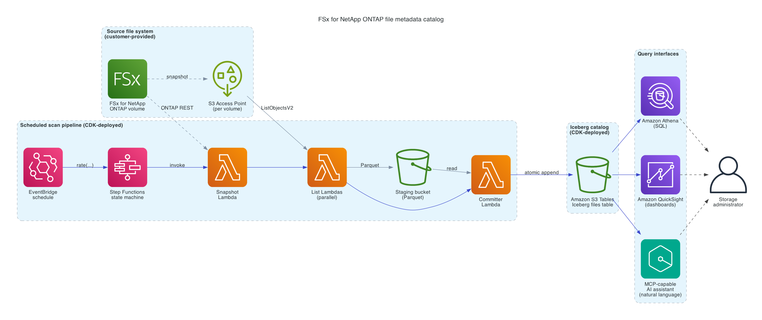
Figure 1: Solution architecture
Each scan of a volume is orchestrated by an AWS Step Functions state machine across three stages:
- An AWS Lambda function calls the ONTAP REST API to create a read-only, point-in-time snapshot of the volume.
- Parallel AWS Lambda functions list the snapshot through the S3 Access Point and capture the metadata for every file — path, size, modification time, ETag, and storage class.
- A final AWS Lambda function reads the per-worker Parquet files from the staging bucket, writes them to the Amazon S3 Tables bucket as a new partition of the Iceberg table, replacing any prior data for the same volume and date in a single atomic transaction, and then deletes the staging Parquet files. The ONTAP snapshot is deleted at the end of the scan.
The result is a single table, partitioned by volume and date, that contains every file on every cataloged volume. Administrators query this table with standard SQL from the Athena console, SDK, or any JDBC/ODBC client.
Key components
The solution uses the following AWS services:
- Amazon FSx for NetApp ONTAP is the source of the file data. The solution operates on existing FSx for NetApp ONTAP volumes and makes no changes to the file system, its clients, or its protocols. It uses two native ONTAP capabilities: read-only volume snapshots, which provide a stable point-in-time view of a volume during each scan; and the ONTAP REST API, which the solution calls to create and delete snapshots.
- Amazon S3 Access Points expose each cataloged volume as an Amazon S3 endpoint, so the solution lists file metadata using the standard S3 ListObjectsV2 API.
- AWS Lambda provides the compute for every stage of a scan. Because Lambda is serverless, the solution incurs minimal compute charges only during active scans.
- AWS Step Functions orchestrates each scan as a state machine. It coordinates the sequence from snapshot creation through commit, runs the listing Lambdas in parallel, and handles retries and error paths automatically.
- Amazon EventBridge triggers scans on a per-volume schedule. Each volume can have its own cadence (for example, hourly for a small active volume, daily for a large archive volume).
- Amazon S3 Tables stores the catalog as an Apache Iceberg table, partitioned by volume and date. S3 Tables provides managed Iceberg storage with built-in compaction and snapshot expiration, so administrators do not have to perform table maintenance themselves.
- Amazon Athena is the query interface. Administrators query the catalog using standard SQL, either from the Athena console, from any JDBC or ODBC client, or from business intelligence tools such as Amazon QuickSight.
- AWS Cloud Development Kit (AWS CDK) packages the solution. The provided CDK application defines all of the above components and deploys them as a single AWS CloudFormation stack containing the shared catalog infrastructure plus one Amazon EventBridge rule per cataloged volume.
Deploy the solution
The solution is packaged as an AWS CDK application that you deploy into your AWS account. Before deploying, you need an Amazon FSx for NetApp ONTAP file system with at least one volume and S3 Access Point, an AWS Secrets Manager secret containing ONTAP administrator credentials for the storage virtual machine, and a VPC subnet and security group for the solution‘s AWS Lambda functions. Detailed prerequisites, including IAM requirements and AWS CLI/CDK version requirements, are listed in the repository README.
To deploy, clone the repository, edit the solution‘s configuration file with your file system ID, volume IDs, Secrets Manager secret ID, and networking details, and run cdk deploy:
git clone https://github.com/aws-samples/sample-fsx-ontap-metadata-catalog
cd sample-fsx-ontap-metadata-catalog/cdk
cdk deploy
The CDK application creates a single AWS CloudFormation stack containing the catalog infrastructure (Amazon S3 Tables bucket, Amazon S3 staging bucket, AWS Lambda functions, AWS Step Functions state machine), plus one Amazon EventBridge rule per cataloged volume. Deployment typically completes in 5 to 10 minutes.
Each volume’s first scheduled scan starts according to the schedule you configured in the configuration file. To populate your catalog immediately rather than waiting for the first scheduled scan, you can trigger an execution of the shared fsx-ontap-catalog-scan state machine for any volume. The CDK application creates this state machine once and shares it across all cataloged volumes; an execution input identifies which volume to scan:
aws stepfunctions start-execution \
  --region <your-region> \
  --state-machine-arn arn:aws:states:<your-region>:<account-id>:stateMachine:fsx-ontap-catalog-scan \
  --input '{
    "volume_name": "<your-volume-name>",
    "s3ap_alias": "<your-volume-s3-access-point-alias>",
    "svm_id": "<your-svm-id>",
    "max_workers": 16,
    "retain_count": 7
  }'
Once the execution succeeds (typically in under a minute for a volume with a few thousand files), your catalog is populated and queryable.
Query your file metadata catalog with Amazon Athena
The catalog is stored as an Apache Iceberg table in Amazon S3 Tables, queryable with standard SQL through Amazon Athena. Once the solution is deployed, the table is available at “s3tablescatalog/fsx-ontap-metadata-catalog”.”catalog”.”files” (quoting is required because the catalog name contains a slash). Because the catalog retains every scheduled scan, the example queries below use a common table expression (CTE) to scope to the most recent scan per volume.
What files are in each of my volumes?
WITH latest AS (
  SELECT volume_name, MAX(dt) AS dt
  FROM "s3tablescatalog/fsx-ontap-metadata-catalog"."catalog"."files"
  GROUP BY volume_name
)
SELECT f.volume_name, COUNT(*) AS file_count,
  ROUND(SUM(f.size_bytes) / POWER(1024, 4), 2) AS total_tib
FROM "s3tablescatalog/fsx-ontap-metadata-catalog"."catalog"."files" f
JOIN latest l ON f.volume_name = l.volume_name AND f.dt = l.dt
GROUP BY f.volume_name
ORDER BY total_tib DESC;
| volume_name | file_count | total_tib |
| home | 94,702 | 3.17 |
| finance | 62,474 | 0.58 |
| engineering | 61,883 | 0.46 |
What kinds of files are stored on each volume?
WITH latest AS (
  SELECT volume_name, MAX(dt) AS dt
  FROM "s3tablescatalog/fsx-ontap-metadata-catalog"."catalog"."files"
  GROUP BY volume_name
)
SELECT f.extension, COUNT(*) AS file_count,
  ROUND(SUM(f.size_bytes) / POWER(1024, 3), 2) AS total_gib
FROM "s3tablescatalog/fsx-ontap-metadata-catalog"."catalog"."files" f
JOIN latest l ON f.volume_name = l.volume_name AND f.dt = l.dt
WHERE f.extension <> ''
GROUP BY f.extension
ORDER BY file_count DESC
LIMIT 10;
Where are files of a specific type located?
WITH latest AS (
  SELECT volume_name, MAX(dt) AS dt
  FROM "s3tablescatalog/fsx-ontap-metadata-catalog"."catalog"."files"
  GROUP BY volume_name
)
SELECT f.volume_name, f.path,
  ROUND(f.size_bytes / POWER(1024, 2), 2) AS size_mib, f.mtime
FROM "s3tablescatalog/fsx-ontap-metadata-catalog"."catalog"."files" f
JOIN latest l ON f.volume_name = l.volume_name AND f.dt = l.dt
WHERE f.extension = 'pst'
ORDER BY f.size_bytes DESC
LIMIT 100;
Which files are the largest?
WITH latest AS (
  SELECT volume_name, MAX(dt) AS dt
  FROM "s3tablescatalog/fsx-ontap-metadata-catalog"."catalog"."files"
  GROUP BY volume_name
)
SELECT f.volume_name, f.path,
  ROUND(f.size_bytes / POWER(1024, 3), 3) AS size_gib,
  f.mtime, f.age_days
FROM "s3tablescatalog/fsx-ontap-metadata-catalog"."catalog"."files" f
JOIN latest l ON f.volume_name = l.volume_name AND f.dt = l.dt
ORDER BY f.size_bytes DESC
LIMIT 100;
The repository’s sql/canned/ directory includes additional starter queries for file age distribution, capacity growth over time, and other common reports.
Query your file metadata catalog in natural language
For administrators who would rather ask questions in plain language than write SQL, the catalog can be queried through an AI assistant such as Amazon Q Developer using the Amazon S3 Tables MCP server. The Model Context Protocol (MCP) is an open protocol that lets AI assistants call external tools; the S3 Tables MCP server exposes read and query operations on your S3 Tables catalogs as tools the assistant can use. Once the MCP server is configured in your client (see the MCP server documentation for setup), you can query the file metadata catalog in natural language.
As a first example, suppose you want a quick overview of how storage is distributed across your volumes. The administrator asks:
“Which of my volumes is using the most storage, and what kinds of files are on it?”
The assistant identifies that this maps to a per-volume aggregation against the most recent scan of each volume and runs:
WITH latest AS (
  SELECT volume_name, MAX(dt) AS dt FROM files GROUP BY volume_name
)
SELECT f.volume_name, COUNT(*) AS file_count,
       ROUND(SUM(f.size_bytes) / POWER(1024, 4), 2) AS total_tib
FROM files f
JOIN latest l ON f.volume_name = l.volume_name AND f.dt = l.dt
GROUP BY f.volume_name
ORDER BY total_tib DESC;
| volume_name | file_count | total_tib |
| home | 94,702 | 3.17 |
| finance | 62,474 | 0.58 |
| engineering | 61,883 | 0.46 |
The assistant summarizes: “Your home volume holds the most data — 3.17 TiB across about 95,000 files, roughly 75% of your total cataloged storage. finance and engineering are similar in file count but much smaller in total size.”
In a single round-trip, the administrator has a complete capacity overview and can decide which volume to focus on next.
For lifecycle and compliance questions, the assistant can combine filtering and aggregation that would be tedious to type in SQL. Suppose the records management team asks about Outlook archive files ahead of a retention review:
“How many .pst files do I have, where are they, and how old are they?”
The assistant runs:
WITH latest AS (
  SELECT volume_name, MAX(dt) AS dt FROM files GROUP BY volume_name
)
SELECT f.volume_name, f.path,
       ROUND(f.size_bytes / POWER(1024, 3), 2) AS size_gib, f.age_days
FROM files f
JOIN latest l ON f.volume_name = l.volume_name AND f.dt = l.dt
WHERE f.extension = 'pst'
ORDER BY f.size_bytes DESC;
| volume_name | path | size_gib | age_days |
| home | /bob/backup/legacy_email.pst | 12.81 | 1839 |
| home | /alice/old_outlook/outlook_2019.pst | 12.81 | 2065 |
| finance | /email_archives/iross/outlook_archive_2019.pst | 11.04 | 2844 |
| finance | /email_archives/bmiller/outlook_archive_2023.pst | 10.33 | 1433 |
| finance | /email_archives/dscott/outlook_archive_2024.pst | 10.22 | 1088 |
| (15 more rows) |
The assistant summarizes: “You have 50+ Outlook archive files. Most are concentrated under finance/email_archives/, organized by user. A few large ones are also in home/ under user directories — for example bob/backup/legacy_email.pst and alice/old_outlook/. Many are 5+ years old (2,000-3,200 days). This is the kind of distribution worth flagging to your records management team.”
The administrator now has a concrete list to act on — both the in-policy archives in finance/email_archives/ and the unexpected copies in user home directories.
Finally, the catalog supports discovery questions that would otherwise require walking the file system. Suppose the storage team wants to identify archival candidates ahead of a quarterly review:
“What are the largest single files in my catalog, and what folders are they in?”
The assistant runs:
WITH latest AS (
  SELECT volume_name, MAX(dt) AS dt FROM files GROUP BY volume_name
)
SELECT f.volume_name, f.path, f.parent_dir,
       ROUND(f.size_bytes / POWER(1024, 3), 2) AS size_gib, f.age_days
FROM files f
JOIN latest l ON f.volume_name = l.volume_name AND f.dt = l.dt
ORDER BY f.size_bytes DESC
LIMIT 15;
| volume_name | path | size_gib | age_days |
| engineering | /images/build-image-035.iso | 27.83 | 968 |
| engineering | /images/macos_dev_env.qcow2 | 26.08 | 408 |
| engineering | /images/build-image-006.vmdk | 25.22 | 81 |
| engineering | /images/build-image-017.vmdk | 24.20 | 629 |
| engineering | /images/build-image-053.ova | 23.10 | 237 |
| (10 more rows) |
The assistant summarizes: “Your largest files are concentrated in two folders. engineering/images/ holds your top 10 by size — VM disk images and ISOs from 16 to 28 GiB. Several are over 18 months old. home/shared/all-hands-recordings/ is your second cluster — quarterly all-hands MP4s at ~16 GiB each, some several years old. If you want to free space, the engineering images folder is where to focus first.”
Without writing any SQL, the administrator has identified specific archival candidates and a clear order of operations.
Two things are worth keeping in mind when using natural-language querying over catalog data. First, the assistant generates the SQL on your behalf, so for queries where accuracy matters — such as audit or compliance reporting — review the SQL that the assistant ran. The assistant surfaces the query, so this is straightforward to verify. Second, the default operating mode of the S3 Tables MCP server is read-only, preventing modifications to the catalog.
Visualize your file metadata catalog with Amazon QuickSight
For administrators who want to share insights with colleagues who don’t write SQL, or who want an always-on dashboard for routine operational review, the catalog can be visualized in Amazon QuickSight. QuickSight connects to the catalog through Amazon Athena and imports it into SPICE for fast, interactive querying. One-time IAM configuration and the dataset setup are documented in the repository README.
Below we demonstrate an example analysis around three common administrator workflows: a current-state overview, a deeper storage-location and lifecycle view, and capacity trends over time. Figure 2 shows the current-state sheet populated with sample data.
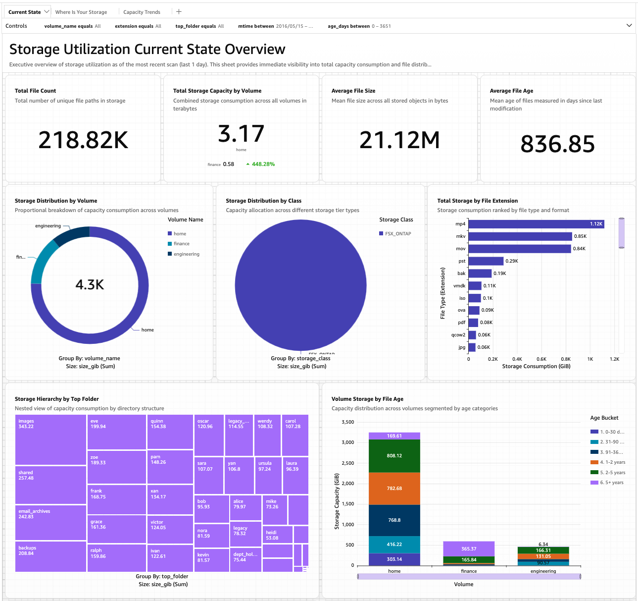
Figure 2: Current-state sheet of the starter QuickSight dashboard.
The current-state sheet is what an administrator opens first thing in the morning: at-a-glance KPIs, capacity distribution across volumes, and the top file types and folders that consume capacity. The same patterns surfaced by the SQL queries earlier appear visually here — video files dominate the top-extensions chart, the home volume holds the bulk of total capacity, and the bottom-right stacked bar reveals that a large share of files are 2-5 years old.
For capacity-driven decisions, the second sheet drills into where data sits and how old it is. Figure 3 shows the storage-location and lifecycle view.
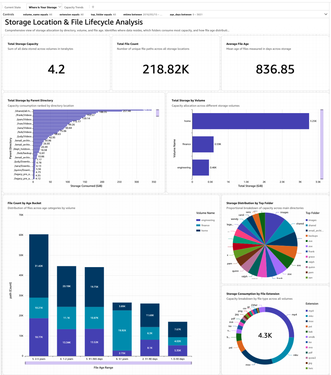
Figure 3: Storage-location and lifecycle sheet, showing top directories by capacity and file count by age bucket per volume.
The horizontal bar chart of top parent directories at upper-left is the visual analogue of the “where is my capacity concentrated?” queries in Athena and the natural-language conversations earlier in this post. The age-bucket stacked bar at lower-left makes lifecycle patterns immediately legible: in this sample data, the 2-5 year bucket on the home volume is the dominant cohort, suggesting a backlog of older content that may be archival-ready.
For long-term planning, the third sheet displays how the catalog is evolving over time — file counts and capacity per volume across scan history.
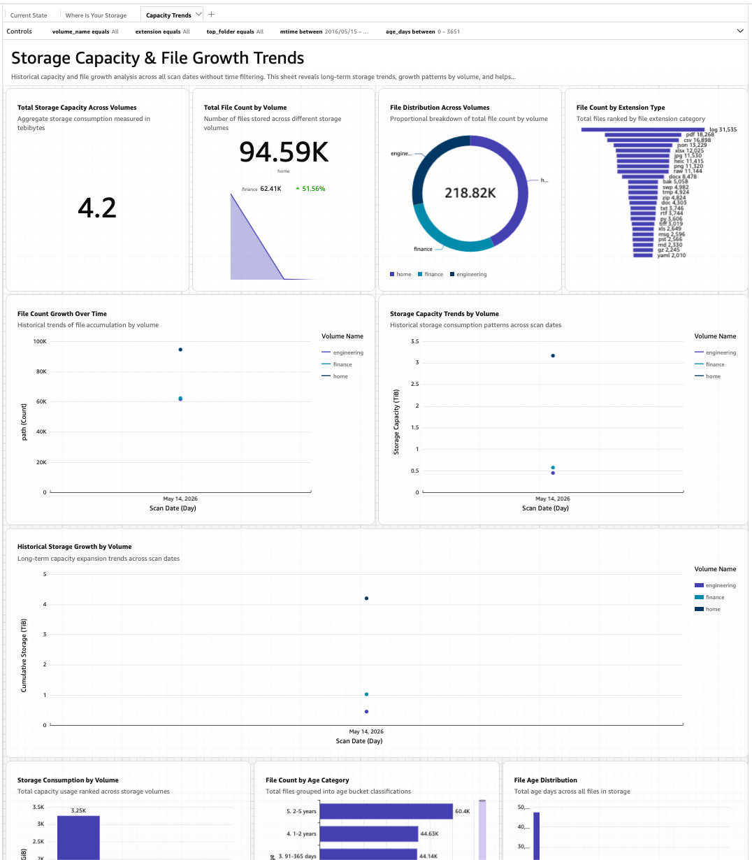
Figure 4: Capacity-trends sheet, showing file counts and capacity per volume across scan history.
Trends become apparent over time that no single point-in-time query can reveal: steady-state versus runaway growth, sudden capacity drops from large deletions, or divergence between volumes that were once similar. Figure 4 shows the sheet shortly after a fresh deployment, when only a single scan exists per volume, so the line and area charts each have one data point. The chart structure is in place; the lines fill in as scheduled scans accumulate over days and weeks.
Because QuickSight dashboards can be shared through email and embedded in external web applications, they are also a natural way to surface file storage insights to stakeholders outside the storage team — finance reviewing cost trends, legal auditing retention, or engineering leadership planning headcount growth.
Clean Up
To remove the solution so as not to incur unwanted charges, run cdk destroy from the same directory. This removes all deployed AWS resources except the Amazon S3 Tables bucket and its contents, which the CDK retains by default to prevent accidental data loss. To remove the catalog data as well, delete the S3 Tables bucket manually after cdk destroy completes.
Conclusion
Understanding what is stored in an enterprise file system is a foundational capability that most storage administrators still lack. The solution described in this post makes that visibility straightforward: a continuously refreshed, SQL-queryable catalog of file metadata for Amazon FSx for NetApp ONTAP, built from standard AWS building blocks — Amazon S3 Access Points for FSx for NetApp ONTAP, AWS Lambda, Amazon S3 Tables, and Amazon Athena — and packaged as an AWS CDK application that deploys in minutes.
Once running, the catalog supports three complementary ways to explore your file data: writing SQL directly in Amazon Athena for precise, reproducible queries; asking natural-language questions through the Amazon S3 Tables MCP server from any MCP-capable AI assistant for ad-hoc discovery; and building dashboards in Amazon QuickSight for ongoing operational review and sharing with colleagues outside the storage team. The three interfaces are additive — the same catalog serves all of them.
This pattern — Iceberg-formatted metadata that any AWS analytics service can query — is the same one that Amazon S3 Metadata brings to general-purpose Amazon S3 buckets. The solution in this post applies the same approach to FSx for NetApp ONTAP file data, using S3 Access Points as the bridge between file storage and the AWS analytics ecosystem.
To get started, visit the aws-samples repository for deployment instructions, starter SQL queries, and the reference QuickSight dashboard.