Accelerating Spark queries with Iceberg materialized views

In this post, you learn how to reduce Apache Spark query execution time with Apache Iceberg materialized views without changing a single SQL query.

Organizations running analytical workloads on their data lakes often hit a common wall: queries that are slow and costly, yet difficult to rewrite by hand. Multi-table joins, heavy aggregations, and window functions over large fact tables all drive up execution times, but the SQL behind them often can’t be changed. It might come from business intelligence (BI) dashboards, packaged independent software vendor (ISV) applications, or legacy reports, where editing the source introduces regression risk that outweighs the performance gain.

Starting with Amazon EMR 7.12.0 and AWS Glue 5.1, you can accelerate these queries without rewriting them. Automatic query rewrite analyzes the logical plan of each incoming query and compares it against a metadata cache of available MVs. When the optimizer finds a materialized view (MV) that satisfies all or part of a query, it rewrites the plan to read from that MV instead of the base tables. Matches can be structural (aggregations and joins) or exact (more complex patterns like window functions). If no MV matches, the original query runs unchanged with no impact on correctness.

If you have previously tried to speed up slow analytical queries, you might have considered one of the following alternatives. Here is how automatic query rewrite compares:

In this post, we:

• Give a high-level overview of how automatic query rewrite works in Apache Spark.
• Walk through a concrete example, showing how the same query can benefit from MVs at different levels of coverage.
• Discuss the trade-offs so you can choose the right MV shape for your workload.

Prerequisites

To use automatic query rewrite with Iceberg materialized views, you need:

• Amazon EMR release 7.12.0 or later, or AWS Glue 5.1 or later.
• Source tables in Apache Iceberg or Parquet format, registered in the AWS Glue Data Catalog, in the same AWS Region and account as the materialized view. Parquet source tables are supported for automatic query rewrite starting with Amazon EMR 7.14.0 and AWS Glue 8.1.
• An Amazon Simple Storage Service (Amazon S3) Tables (a capability of Amazon S3) bucket, or an S3 general purpose bucket, for the materialized view data.
• Permissions for the definer role. You can use AWS Identity and Access Management (IAM) policies or AWS Lake Formation.
• Automatic query rewrite turned on in your Spark session: --conf spark.sql.optimizer.answerQueriesWithMVs.enabled=true.
• For Parquet source tables, set spark.sql.materializedView.v1SourceTables.enabled=true and spark.sql.materializedView.v1ETagVersioning.enabled=true.

For more Spark configurations, see Introducing Apache Iceberg materialized views in AWS Glue Data Catalog.

How it works

Here is how MVs and automatic query rewrite work together:

• You define a SQL query with aggregations, joins, or filters across your supported source tables.
• AWS Glue Data Catalog stores the precomputed results as an Apache Iceberg table in your Amazon S3 bucket. You can store it in a general purpose S3 bucket or in Amazon S3 Tables. Any Apache Iceberg-compatible query engine can read the materialized view, including Amazon Athena, Amazon EMR, AWS Glue, Amazon Redshift, and Iceberg-compatible third-party query engines. Automatic query rewrite is available on the AWS optimized Spark runtime in Amazon Athena, Amazon EMR, and AWS Glue. Other engines can query the materialized view directly, but they don’t rewrite queries to use it automatically.
• Automatic refresh keeps the MV current on a schedule that you define, for example SCHEDULE REFRESH EVERY 1 DAY. You set it at creation time or later with ALTER MATERIALIZED VIEW ... ADD SCHEDULE REFRESH. At that scheduled time, the refresh process checks the current Apache Iceberg snapshot ID or Parquet file ETags and refreshes the MV when it detects source-table changes.
• Automatic query rewrite redirects matching queries to the MV at query optimization time. Automatic query rewrite in Apache Spark uses two matching strategies:
  • Structural rewrite (adapted from Amazon Redshift) handles an MV defined as a single SELECT-FROM-WHERE-GROUP-BY block over INNER joins. The optimizer can roll up an MV’s aggregates to a coarser grain and pull extra query predicates up onto the MV scan.
  • Exact-match rewrite handles MVs defined as other shapes, such as window functions and outer joins, by matching a canonicalized form of the MV body against subtrees of the query plan.

When the optimizer evaluates a query, it consults a metadata cache of MVs from the configured catalogs and chooses the best match. It also checks MV staleness during optimization. It skips stale MVs, so rewrite won’t return stale results. If no MV matches, the original query runs unchanged.

Note that automatic query rewrite is opt-in: set spark.sql.optimizer.answerQueriesWithMVs.enabled=true when creating the Apache Spark session.

Example: One query with three potential MVs

An MV doesn’t need to cover an entire query to help it. Automatic query rewrite in Apache Spark operates on subtrees: when an MV matches a portion of your query plan, the rewriter substitutes that subtree and lets the rest of the query run on the rewrite output unchanged. The same query can therefore be served by many possible MV designs, each making a different trade-off between per-query speedup, storage cost, and reuse across other queries.

To make this concrete, consider a typical analytics query: “Top 100 preferred US customers by total store spending.” It joins fact and dimension tables, applies two selective filters on the customer dimension, aggregates per customer, ranks the result with a window function, and keeps only the top 100:

SELECT c_customer_id, total_revenue, num_transactions, avg_purchase, revenue_rank
FROM (
    SELECT cust.c_customer_id,
        SUM(sales.ss_quantity * sales.ss_sales_price) AS total_revenue,
        COUNT(*) AS num_transactions,
        AVG(sales.ss_quantity * sales.ss_sales_price) AS avg_purchase,
        RANK() OVER (ORDER BY SUM(sales.ss_quantity * sales.ss_sales_price) DESC) AS revenue_rank
    FROM base_catalog.base_db.store_sales sales
    INNER JOIN base_catalog.base_db.customer cust
        ON sales.ss_customer_sk = cust.c_customer_sk
    WHERE cust.c_birth_country = 'UNITED STATES'
        AND cust.c_preferred_cust_flag = 'Y'
    GROUP BY cust.c_customer_id
) ranked
WHERE revenue_rank <= 100
ORDER BY revenue_rank;

Query 1: The original query. Top 100 preferred US customers by total store spending, before any materialized view.

Three MV designs cover progressively more of this query, from a single-table pre-aggregate to the full query body itself:

Tier 1: Pre-aggregate store_sales only, no join, no filter. This tier is a single-table aggregate of store_sales at customer-surrogate-key grain. The query still must join the customer table, apply both filters, re-aggregate at c_customer_id grain, and run the window function.

CREATE MATERIALIZED VIEW mv_catalog.mv_db.customer_tier_1 AS
SELECT ss_customer_sk,
    SUM(ss_quantity * ss_sales_price) AS sum_revenue,
    COUNT(ss_quantity * ss_sales_price) AS count_revenue,
    COUNT(*) AS num
FROM base_catalog.base_db.store_sales
GROUP BY ss_customer_sk;

Tier 1 MV: Single-table pre-aggregate of store_sales by customer surrogate key (no join, no filter).

The following plans compare the original query plan to the rewritten plan:

Window, filter, Sort
+- Aggregate by c_customer_id
:  total_revenue = SUM(ss_quantity * ss_sales_price)
:  num_transactions = COUNT(*)
:  avg_purchase = AVG(ss_quantity * ss_sales_price)
+- Project
   +- Join Inner ON ss_customer_sk = c_customer_sk
      :- BatchScan store_sales <- reads the large store_sales table
      +- Filter c_birth_country='UNITED STATES' AND c_preferred_cust_flag='Y'
         +- BatchScan customer

Plan 1: Original plan. Scans the large store_sales table.

Window, filter, Sort
+- Aggregate by c_customer_id <- rolls up pre-aggregated sums
:  total_revenue = SUM(sum_revenue) <- sum of sum_revenue
:  num_transactions = SUM(num) <- sum of num
:  avg_purchase = SUM(sum_revenue) / SUM(count_revenue) <- sum of sum_revenue / sum of count_revenue
+- Project
   +- Join Inner ON ss_customer_sk = c_customer_sk
      :- BatchScan customer_tier_1 <- reads pre-aggregated MV
      +- Filter c_birth_country='UNITED STATES' AND c_preferred_cust_flag='Y'
         +- BatchScan customer

Plan 2: Rewritten plan (Tier 1). Reads the pre-aggregated customer_tier_1 MV.

Tier 2: Pre-join store_sales x customer, pre-apply one filter (c_preferred_cust_flag = ‘Y’). The middle tier pre-joins both tables and bakes in the preferred-customer filter. The query still must apply the country filter as a residual on the MV scan and run the RANK() window.

CREATE MATERIALIZED VIEW mv_catalog.mv_db.customer_tier_2 AS
SELECT cust.c_customer_id, cust.c_birth_country,
    SUM(sales.ss_quantity * sales.ss_sales_price) AS sum_revenue,
    COUNT(sales.ss_quantity * sales.ss_sales_price) AS count_revenue,
    COUNT(*) AS num
FROM base_catalog.base_db.store_sales sales
INNER JOIN base_catalog.base_db.customer cust
    ON sales.ss_customer_sk = cust.c_customer_sk
WHERE cust.c_preferred_cust_flag = 'Y'
GROUP BY cust.c_customer_id, cust.c_birth_country;

Tier 2 MV: Pre-joins store_sales and customer, with the preferred-customer filter applied.

Rewritten query plan:

Window, filter, Sort
+- Aggregate by c_customer_id <- rolls up pre-aggregated sums
:  total_revenue = SUM(sum_revenue) <- sum of sum_revenue
:  num_transactions = SUM(num) <- sum of num
:  avg_purchase = SUM(sum_revenue) / SUM(count_revenue) <- reads pre-aggregated MV
+- Filter c_birth_country='UNITED STATES' [residual filter on MV scan]
   +- BatchScan customer_tier_2 <- reads pre-aggregated MV

Plan 3: Rewritten plan (Tier 2). Country filter applied as a residual on the MV scan.

Tier 3: Match the entire query, including the window function and top N filter. This is the most specific tier. The MV body is the target query verbatim (minus the top-level ORDER BY, which is meaningless for a stored set). The MV stores the top-ranked rows the query asks for (rank ≤ 100).

CREATE MATERIALIZED VIEW mv_catalog.mv_db.customer_tier_3 AS
SELECT c_customer_id, total_revenue, num_transactions, avg_purchase, revenue_rank
FROM (
    SELECT cust.c_customer_id,
        SUM(sales.ss_quantity * sales.ss_sales_price) AS total_revenue,
        COUNT(*) AS num_transactions,
        AVG(sales.ss_quantity * sales.ss_sales_price) AS avg_purchase,
        RANK() OVER (ORDER BY SUM(sales.ss_quantity * sales.ss_sales_price) DESC) AS revenue_rank
    FROM base_catalog.base_db.store_sales sales
    INNER JOIN base_catalog.base_db.customer cust
        ON sales.ss_customer_sk = cust.c_customer_sk
    WHERE cust.c_birth_country = 'UNITED STATES'
        AND cust.c_preferred_cust_flag = 'Y'
    GROUP BY cust.c_customer_id
) ranked
WHERE revenue_rank <= 100;

Tier 3 MV: Stores the exact ranked output of the query (exact-match path).

This tier exercises the exact-match rewrite path: the rewriter canonicalizes the MV body and matches it against the query’s logical plan.

Rewritten plan:

Sort revenue_rank ASC
+- BatchScan customer_tier_3 <- reads around 100 stored rows

Plan 4: Rewritten plan (Tier 3). Reads around 100 stored rows.

The trade-off

The three tiers trade per-query speedup against reuse and storage. In our testing on TPC-DS 3 TB, we observed the following:

Performance measured on TPC-DS 3 TB. Speedup is the ratio of baseline execution time to MV-accelerated execution time. Results might vary based on data characteristics, cluster size, and query complexity.

In addition, MVs incur additional cost. Each one runs a query against your source tables once and stores the result. The more pre-computation it does (joining more tables, applying more filters), the more time it takes.

The following chart plots per-query speedup and creation time for the three tiers in our testing on TPC-DS 3 TB. Per-query speedup rises steadily, from about 5x at Tier 1 to over 20x at Tier 3. Creation time doesn’t follow the same pattern: it peaks at Tier 2. Tier 2 pre-joins and aggregates all preferred customers across every country, so it materializes the most data work. Tier 3 applies both filters, so it processes far fewer rows and costs less to create.

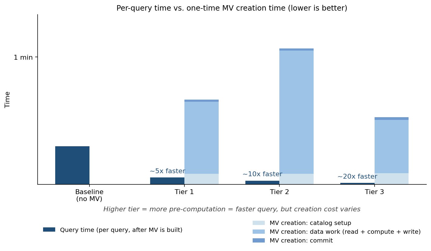
Figure 1: Per-query speedup and creation time across the three materialized view tiers, measured on TPC-DS 3 TB

Start by identifying one expensive query that runs repeatedly with stable filters. It is likely a good candidate for an exact-match MV.

Validating automatic query rewrite

To confirm that your query benefited from automatic rewrite:

1. Query plan inspection: Check the query’s optimized logical plan or physical plan for a leaf scan node referencing the MV (for example, BatchScan mv_catalog.mv_db.your_mv_name). If the MV appears as a scan source, rewrite succeeded.
2. Log confirmation (Amazon EMR 7.14.0+): Look for INFO-level log entries such as AQMV outcome: rewritten=true, mvs=[mv_name], duration=12ms.
3. No-rewrite diagnostics (Amazon EMR 7.14.0+): If rewrite didn’t occur, check the MVRewriteMetricsEvent in the Apache Spark Event Log for the specific reason the optimizer skipped the MV.

If you have set spark.sql.optimizer.answerQueriesWithMVs.enabled=true but your query still runs against the base tables, check the following common causes:

1. Write commands block rewrite by default. INSERT and MERGE statements don’t trigger rewrite. Set spark.sql.optimizer.answerQueriesWithMVs.commandBlockingEnabled=false to turn on rewrite within write command subqueries.
2. The MV is stale. Rewrite skips the MV when one or more source tables have changed since its last refresh. Wait for the next scheduled refresh, or force an immediate refresh with REFRESH MATERIALIZED VIEW <mv_name>.
3. Heuristic candidate filtering. The optimizer uses heuristic checks to narrow the set of MV candidates before attempting a full match. In some cases, an MV that could benefit the query might be filtered out early by these heuristics.
4. Spark version mismatch (Amazon EMR 7.13.0+). Automatic query rewrite skips MVs whose stored IMV_sparkVersion does not match the cluster’s current Apache Spark version. To bypass this check, set spark.sql.materializedView.sparkVersionCompatibilityCheck.enabled=false.
5. MV metadata cache not loaded. The metadata cache loads lazily during optimization of the first rewritable query in a Spark session. If your critical query fires before the cache is warm, the MV will not be available. Run a small warm-up query (for example, SELECT 1 FROM <some_iceberg_table>) at session start to pay this cost off the critical path.
6. MV metadata cache memory limit reached. If the cache was disabled or stopped loading MVs because of reaching its memory limit, increase spark.driver.memory.
7. Too many tables in configured catalogs. If there are many tables or MVs in the configured catalogs, the cache might not finish loading before your query starts. Place MVs in a dedicated catalog, add it to spark.sql.materializedViews.additionalCatalogs, and set spark.sql.materializedViews.scanCurrentCatalog=false to skip scanning the current catalog.
8. Parquet base tables have additional limitations and configuration requirements. For automatic query rewrite with Parquet base tables, set spark.sql.materializedView.v1SourceTables.enabled=true and spark.sql.materializedView.v1ETagVersioning.enabled=true. Without ETag versioning, Spark can’t determine a usable source-table version and skips the MV. Partitioned Parquet base tables are also subject to additional validation limits.

Performance considerations

Turning on automatic query rewrite has overhead: it introduces trade-offs that might affect some queries negatively:

1. Optimization overhead. Enabling rewrite adds processing time during query optimization as the optimizer evaluates MV candidates against the query plan. This overhead applies to every query in the session, including those that ultimately don’t match any MV.
2. Reduced task parallelism. Reading from an MV instead of the original base table might produce fewer tasks or introduce data skew, depending on the MV’s data layout. This reduces parallelism compared to a direct scan of the larger, more evenly distributed source table.

Conclusion

In this post, we showed how automatic query rewrite can accelerate your existing Apache Spark workloads. It uses Apache Iceberg materialized views in the AWS Glue Data Catalog, without changing a single line of SQL. By storing precomputed results as managed Apache Iceberg tables, the AWS Glue Data Catalog lets the Apache Spark optimizer transparently substitute matching query plans. You get the performance benefit of pre-aggregation without the application-level rewiring. BI dashboards, ISV-generated reports, and legacy pipelines all benefit the moment a matching MV exists.

We walked through three MV designs for the same analytical query, each striking a different balance between per-query speedup, storage footprint, and reuse across your workload. As the trade-off table shows, our testing found that a narrow, exact-match MV delivered 20x+ acceleration for a single query shape. A broader pre-aggregate served an entire family of queries at a more modest ~5x gain. The right choice depends on how many queries share the same join-and-aggregate pattern and how frequently your source data changes.

To get started:

1. Launch an Amazon EMR 7.12.0+ cluster or an AWS Glue 5.1+ job.
2. Create an MV over your most expensive repeating query using CREATE MATERIALIZED VIEW in the AWS Glue Data Catalog.
3. Turn on automatic query rewrite by setting spark.sql.optimizer.answerQueriesWithMVs.enabled=true in your Spark session configuration.
4. Verify the rewrite by inspecting the optimized query plan for an MV scan node, or by checking INFO-level logs on Amazon EMR 7.14.0+.

Queries with multi-table joins, heavy aggregations, or window functions over large fact tables are strong initial candidates. Start with one high-cost, frequently executed query. Validate the speedup, then expand to broader MVs as you identify shared patterns across your workload.

Special thanks to everyone who contributed to the automatic query rewrite feature and this blog: Andre Hernich, Leon Lin, Yiyang Chen, Geeta Krishna Panda, Ashok Chintalapati, Muhammad Malik, Rishabh Bhatia, and Giovanni Fumarola.

References

For more detail, see the following resources:

• Using materialized views with Amazon EMR.
• Using materialized views with AWS Glue.
• Querying materialized views in Amazon Athena.
• Introducing Apache Iceberg materialized views in AWS Glue Data Catalog.
• Materialized views in AWS Lake Formation.
• How to use streamlined permissions for Amazon S3 Tables and Iceberg materialized views.

About the authors