Build a real-time event pipeline with Spark Real-Time Mode on AWS Glue 6.0

Real-time event pipelines rarely get to work with a uniform schema. Whether it’s IoT metrics, ecommerce clickstreams, or financial pricing vectors, each event type brings its own schema. An equity trade and a rates trade, for instance, carry almost entirely different fields. Ingesting these multi-schema streams has traditionally forced suboptimal architectural choices. You build separate tables for each event type or maintain a wide STRUCT where every possible field across all event types must be declared upfront (fast reads, but sparse and rigid). The other option is to flatten everything into an unwieldy schema with hundreds of columns. To sidestep that maintenance burden, many teams dump events into a plain JSON string column that introduces significant performance penalty. Querying a single nested field requires your engine to deserialize the entire JSON blob for every row. At scale, you burn compute and budget scanning terabytes of raw text to extract a few bytes of data.

Adding to the challenge, these pipelines typically demand mixed processing speeds. You need a real-time path (not near-real-time) to flag anomalies or high-risk events with sub-second latency, while simultaneously pushing those same events into analytical storage for deep historical analysis in batch.

With AWS Glue 6.0, you can tackle all of these challenges (schema heterogeneity, JSON scanning overhead, and mixed-latency requirements) from a single pipeline. Built on Apache Spark 4.1 with Apache Iceberg v3 support, AWS Glue 6.0 brings Variant columns, Variant shredding, Spark Real-Time Mode (RTM), and Arrow-native user-defined functions (UDFs) to a fully managed, serverless environment.

In this post, we walk you through how to build this multi-layer architecture using a financial services use case: a market risk pipeline processing trade pricing vectors. While the example is finance, the patterns apply wherever you deal with heterogeneous schemas, expensive JSON parsing, and mixed real-time/batch requirements such as IoT device fleets, multi-tenant SaaS platforms, logistics tracking, and beyond. We will show you how to flag high-risk trades with sub-second latency, stream everything into an Iceberg v3 data lake as Variants, and run batch Value at Risk (VaR) computations efficiently using Arrow-native UDFs.

Solution overview

A bank’s Market Risk team receives a continuous stream of trade pricing vectors from front-office systems. Each trade event carries:

1. A trade ID and book/desk IDs.
2. A pricing vector as semi-structured data. The schema varies by asset class (for example, equities carry risk sensitivities known as Greeks such as delta/gamma, foreign exchange (FX) carries volatility surfaces, rates carry curve sensitivities).
3. A region ID for jurisdictional reporting (uses a column DEFAULT value, so rows that omit it get auto-populated).

The team needs three things from this stream, each at a different speed. We build the pipeline in three layers, each addressing a distinct requirement with a purpose-built AWS Glue 6.0 capability.

Layer 1: Real-time trade position breach detection (sub-second latency)

Positions must be updated in sub-second time, not seconds of traditional micro-batch streaming. For a team monitoring position limits, those seconds mean trades can breach limits before the system reacts. Spark Real-Time Mode (RTM) eliminates the micro-batch boundary entirely, letting records flow continuously through the pipeline so that high-risk trades trigger alerts within sub-second latency of arrival.

Layer 2: Near-real-time analytical lakehouse (seconds latency)

Every trade must land in a queryable data lake within seconds, with heterogeneous pricing vectors stored without declaring a fixed schema upfront. The Iceberg v3 Variant type handles this natively. The raw semi-structured payload goes into a single column regardless of asset class schema. At write time, Variant shredding automatically extracts fields observed in the data into typed Parquet columns, so downstream analytical queries read only the columns they need without deserializing the full blob. Trade amendments and cancellations are handled at a lower cost with deletion vectors (merge-on-read), and column DEFAULT values reduce boilerplate in ingestion code.

Layer 3: Batch risk computation (minutes to hours latency)

Risk metrics like Value at Risk (VaR) must be computed in Python across millions of trades. Traditional row-by-row pickle serialization between the Java Virtual Machine (JVM) and Python is the bottleneck. Arrow-native UDFs process data as vectorized columnar batches, eliminating serialization overhead and accelerating Python-based risk calculations.

The solution uses three separate AWS Glue 6.0 jobs, each independently scalable:

• Real-time path (Scala, gluestreaming): Reads trades from Amazon Managed Streaming for Apache Kafka (Amazon MSK), enriches them with risk scores and breach flags, and writes alerts to a downstream Kafka topic. It runs with a fixed set of workers that are always on. Downstream fraud detection and position limit systems consume the alerts topic for real-time blocking decisions.
• Near-real-time path (PySpark, gluestreaming): Reads from the same MSK topic and lands the full trade history into an Iceberg v3 table. It uses Glue auto scaling and can scale down between batches, keeping costs lower.
• Batch analytics (PySpark, glueetl): Reads from the Iceberg v3 table, extracts fields using variant_get, computes VaR across the portfolio, and writes aggregated risk reports to a downstream summary table.

The following diagram illustrates the solution architecture.

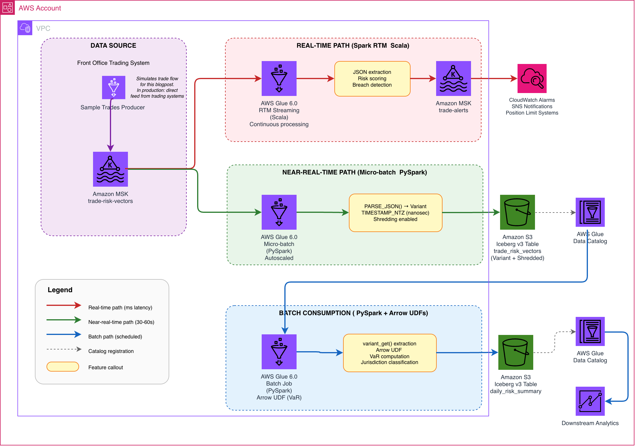
Figure 1: Real-time market risk pipeline on AWS Glue 6.0

Prerequisites

To follow along with this post, you need the following:

1. An AWS account in a Region where AWS Glue 6.0 is available.
2. An AWS Identity and Access Management (IAM) role with permissions to deploy AWS CloudFormation stacks and create resources including AWS Glue, Amazon MSK, AWS Lambda, Amazon Simple Storage Service (Amazon S3), and the AWS Glue Data Catalog.

Deploy the CloudFormation stack

We provide an AWS CloudFormation template that provisions all the resources needed for this walkthrough.

The stack provisions the following resources:

• An Amazon MSK cluster with two topics: trade-risk-vectors (input) and trade-alerts (real-time alerts output).
• An Amazon S3 bucket for Iceberg table storage and streaming checkpoints.
• An AWS Glue database (risk_analytics_<account-id>_glue6b1).
• An IAM role (GlueRole-<account-id>-glue6b1) with permissions for Glue, MSK, S3, and CloudWatch.
• Virtual private cloud (VPC) networking: A Glue network connection (connection-<account-id>-glue6b1), S3 gateway endpoint, and Glue interface endpoint.
• AWS Glue job rtm-alerts-<account-id>-glue6b1 (Scala): This job reads trades from MSK, scores risk in real time using Spark RTM, writes alerts to the trade-alerts topic.
• AWS Glue job nrt-ingestion-<account-id>-glue6b1 (PySpark): This job reads trades from MSK, writes to Iceberg v3 table with Variant + shredding enabled.
• AWS Glue job batch-var-<account-id>-glue6b1 (PySpark): This job reads from Iceberg v3 table, computes VaR with Arrow UDF, demonstrates deletion vectors.
• AWS Glue job producer-<account-id>-glue6b1-helper (PySpark): This job generates sample trade events (equities, FX, rates) to the trade-risk-vectors topic.

Deploy the CloudFormation stack:

1. Download the CloudFormation template from the GitHub repository.
2. Sign in to the AWS CloudFormation console
3. Choose Create stack > With new resources > Upload a template file, and upload the downloaded template.
4. Enter the following parameters:
   • VpcId: Your VPC ID.
   • SubnetIds: At least two subnets in different Availability Zones.
   • SecurityGroupId: A dedicated security group that allows all inbound TCP traffic from itself (self-referencing rule).
   • RouteTableId: The main route table for your VPC.
5. Acknowledge the IAM capabilities and choose Create stack.

Stack creation takes approximately 20 minutes.

After the stack completes, open the AWS Glue console and start the jobs in this order:

1. Start rtm-alerts-<account-id>-glue6b1 and nrt-ingestion-<account-id>-glue6b1.
2. Once both show RUNNING, start producer-<account-id>-glue6b1-helper.
3. After the producer finishes (~3.5 minutes), run batch-var-<account-id>-glue6b1 for risk aggregation.

The consumers must be running before the producer starts so that trades are scored in real time and landed in the Iceberg table as they arrive. The batch job runs last because it reads from the Iceberg table that the near-real-time path populates.

Understand the Iceberg v3 table design

The CloudFormation stack provisions Glue jobs that create two Iceberg v3 tables, trade_risk_vectors (primary trade store) and daily_risk_summary (batch VaR output), using new data types and features:

1. VARIANT: Stores semi-structured pricing vectors without requiring a fixed schema.
2. DEFAULT values: Automatically applies provided defaults when fields aren’t provided.
3. Deletion vectors (merge-on-read): Enables fast row-level updates and deletes.

Open the AWS Glue console under Data Catalog > Tables > trade_risk_vectors.

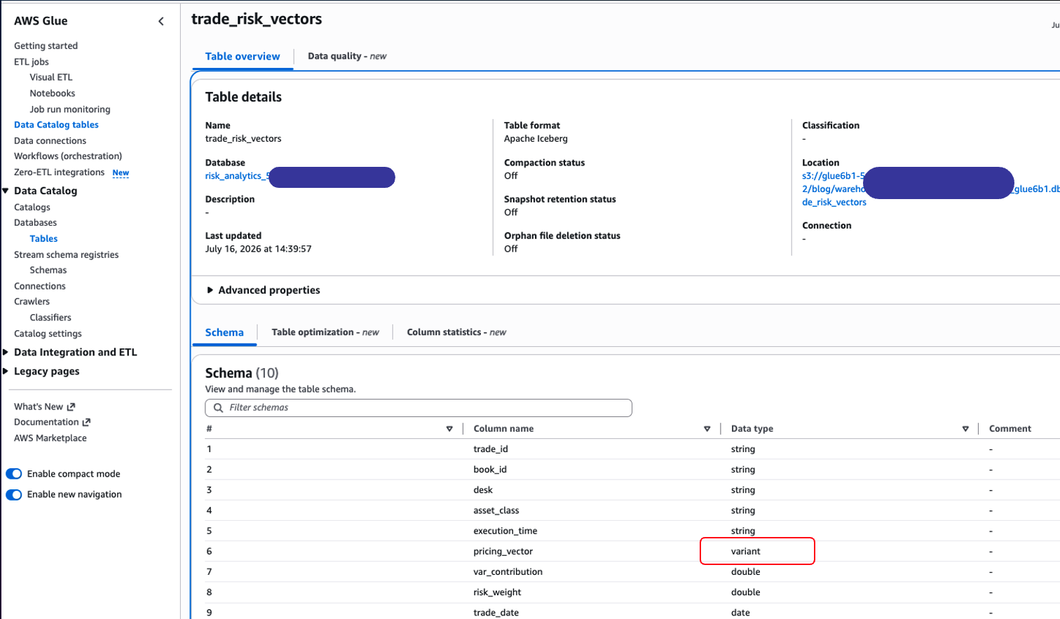
Figure 2: The trade_risk_vectors table in the AWS Glue Data Catalog

The following is the Create Table command:

CREATE TABLE {TABLE} (
    trade_id STRING, book_id STRING, desk STRING,
    asset_class STRING DEFAULT 'UNKNOWN',
    execution_time STRING,
    pricing_vector VARIANT,
    var_contribution DOUBLE DEFAULT 0.0,
    risk_weight DOUBLE DEFAULT 1.0,
    trade_date DATE, region STRING DEFAULT 'EMEA'
) USING iceberg
TBLPROPERTIES ('format-version'='3', 'write.delete.mode'='merge-on-read',
    'write.update.mode'='merge-on-read',
    'write.parquet.shred-variants'='true')
PARTITIONED BY (trade_date, asset_class)

Note the use of DEFAULT values for asset_class, var_contribution, risk_weight, and region. This is an Iceberg v3 feature that applies defaults automatically when values aren’t provided during writes, reducing boilerplate in ingestion code. The pricing_vector column is defined as a Variant type, and write.parquet.shred-variants='true' automatically extracts Variant fields into separate typed Parquet columns at write time for faster downstream queries.

Sample trade event generator

The CloudFormation stack includes a Glue job (producer-<accountid>-glue6b1-helper) that produces realistic trade events to the trade-risk-vectors MSK topic. Each event carries a pricing_vector with a completely different schema per asset class. This is exactly the problem Variant solves.

Equity trade (greeks, scenarios with sector/region breakdowns):

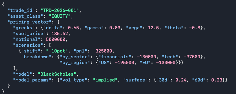
Figure 3: Sample equity trade pricing vector

Rates trade (curve sensitivities per tenor, calibration params):

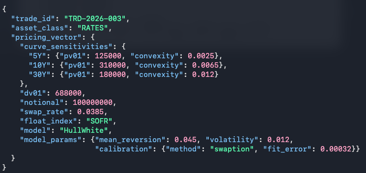
Figure 4: Sample rates trade pricing vector

Completely different structures: greeks vs curve sensitivities, BlackScholes vs HullWhite. Both land in the same pricing_vector VARIANT column with no schema changes required.

Ingest trades with Spark Real-Time Mode

Traditional Spark Structured Streaming uses micro-batches: collect records, schedule a job, process, commit, wait. Even with small batches, the fixed overhead of planning and scheduling adds noticeable latency per batch. For a risk team monitoring position limits, the delay can let a trade breach a limit before the system reacts.

The following Scala job reads trade events from Amazon MSK, applies lightweight risk rules based on data directly available in the event, and writes alerts to a Kafka topic, all with sub-second latency. The real-time path intentionally avoids external lookups (market data, volatility surfaces) to stay fast. The full VaR computation happens later in the batch layer where latency is less critical.

You can view the complete job code in the AWS Glue console under the rtm-alerts-<accountid>-glue6b1 job. Additionally, all the scripts are available in the GitHub repository.

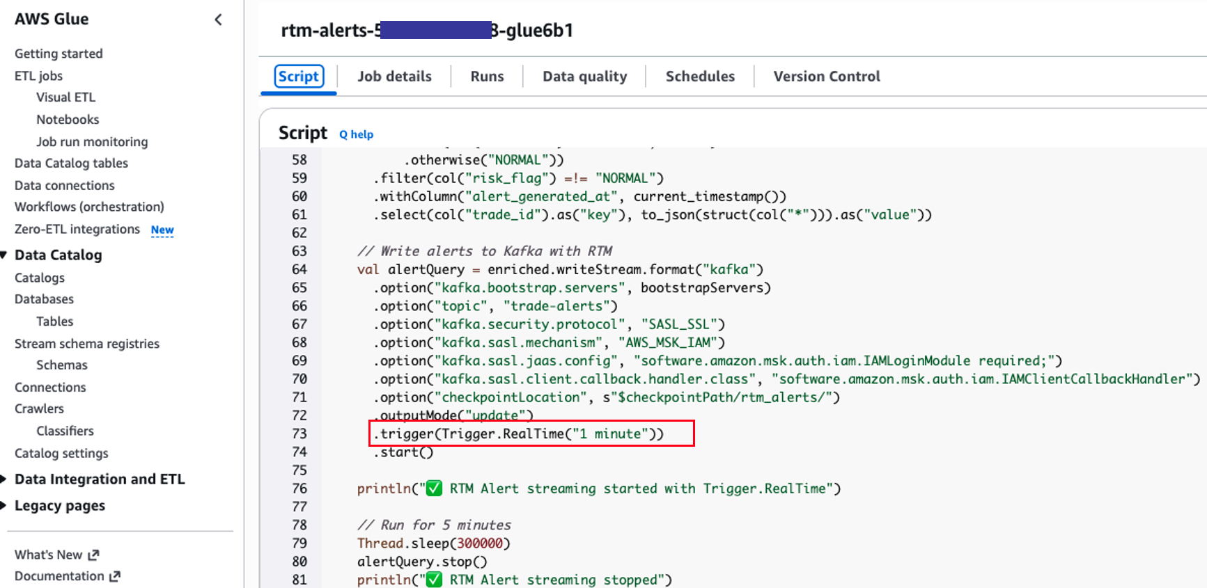
Figure 5: Scala real-time job that scores trades and writes alerts

The Trigger.RealTime("1 minute") is what distinguishes this from a traditional micro-batch. Records flow through the pipeline continuously. Records are processed the instant they arrive. The 1-minute parameter controls how often Spark checkpoints its progress for recovery. It does not control how often records are processed. RTM on AWS Glue 6.0 currently supports Kafka-source, stateless, Scala workloads with fixed workers (no auto scaling) and update output mode only. This makes it ideal for stateless transformations that require sub-second latency, such as the filter, enrich, score, and route pattern shown here. The heavier computation (VaR, aggregations) runs in the micro-batch/batch layer where sub-second latency is less critical.

The real-time path acts as a circuit breaker: trades over $50M notional are flagged CRITICAL, over $25M flagged HIGH. Downstream systems consume the trade-alerts topic and can block or escalate before the next trade executes. The detailed VaR computation (which requires market data, volatility surfaces, and the full pricing vector) runs in the batch consumption layer where latency is less sensitive.

After the streaming phase completes, the job reads back from the trade-alerts topic and measures end-to-end latency. It compares two MSK timestamps: when the trade was received by MSK from the producer, and when the alert was received by MSK from RTM.

To verify the alerts and latency, open the Amazon CloudWatch console > Log groups > /aws-glue/jobs/output and select the RTM job’s log stream. You will see the alert summary showing each flagged trade with its end-to-end latency. The following is a sample.

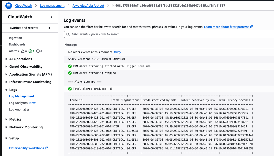
Figure 6: CloudWatch output showing flagged trades and end-to-end latency

Store trades in Iceberg v3 with Variant shredding enabled

The near-real-time path reads from the same MSK topic but writes to an Iceberg v3 table using standard micro-batch streaming. This job runs separately with auto scaling enabled, scaling between batches, keeping costs lower than the always-on real-time path.

You can view the complete job code in the AWS Glue console under the nrt-ingestion-<accountId>-glue6b1 job. The critical aspects are the Variant conversion and the Iceberg write:

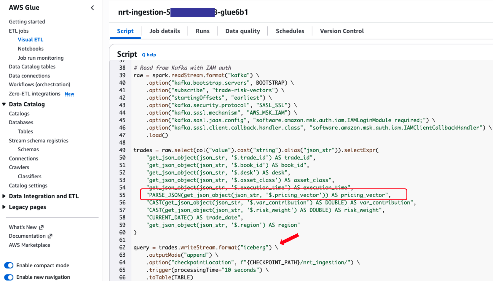
Figure 7: Near-real-time PySpark job writing trades to Iceberg v3 as a Variant

The PARSE_JSON() function converts the raw pricing vector into a native Variant, regardless of the asset class schema. Whether the incoming trade is an equity with greeks, an FX option with a volatility surface, or a rates swap with curve sensitivities, it all goes into the same column. Since the table has write.parquet.shred-variants enabled, fields observed in the initial sample are automatically extracted into typed Parquet columns for fast downstream queries.

How shredding works

During the write process, Spark automatically extracts the Variant fields it observes into separate typed Parquet columns at write time, a feature called shredding. At the start of each write, the engine buffers a sample of rows (controlled by write.parquet.variant-inference-buffer-size), infers which fields exist and their types, then uses that schema to shred all subsequent rows in the file. Every field observed in that sample gets its own typed column, including nested objects. Rows that lack a particular field simply store NULL in that shredded column. For our risk table, fields like $.greeks.delta, $.dv01, and $.model all live in their own typed Parquet columns, even if only one asset class carries a specific field. The result: faster read performance because queries access only the typed columns they need, skipping the rest of the document entirely. Shredding is transparent to queries. variant_get() calls work the same way whether the field is shredded or not. The query engine automatically routes to the shredded column when available, falling back to the binary Variant blob for fields that aren’t part of the inferred schema.

Note: Shredding adds write latency because the engine must infer the schema and write additional typed columns. In this pipeline, we enable shredding on the near-real-time path and absorb that cost, since the downstream read benefits (batch VaR, ad-hoc queries, audit) far outweigh the write penalty. For latency-sensitive pipelines where every millisecond on the write path matters, you can disable shredding on the streaming table and instead write shredded data in a separate batch job that reads from the unshredded table and inserts into a shredded copy. This approach trades architectural simplicity for lower ingestion latency.

Build the batch consumption layer

The third AWS Glue 6.0 job reads from the Iceberg v3 table, extracts risk metrics from the Variant column, computes VaR using an Arrow-native UDF, and writes aggregated results to a summary table.

You can view the complete job code in the AWS Glue console under the batch-var-<accountid>-glue6b1 job. The key aspects are the variant_get extraction from deeply nested structures and the Arrow-native UDF:

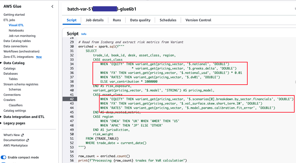
Figure 8: Extracting nested Variant fields with variant_get

Notice how variant_get reaches into arbitrarily nested structures: $.greeks.delta (2 levels), $.scenarios[0].breakdown.by_sector.financials (5 levels), $.model_params.calibration.fit_error (4 levels). All with the same function call. No pre-flattening, no schema-per-asset-class tables, no ETL to restructure the data before querying.

Once the risk metrics are extracted, we need to run a Monte Carlo-style Historical VaR that simulates 1,000 daily profit and loss (P&L) scenarios per trade and returns the 99th percentile loss. This is where the @arrow_udf decorator comes in.

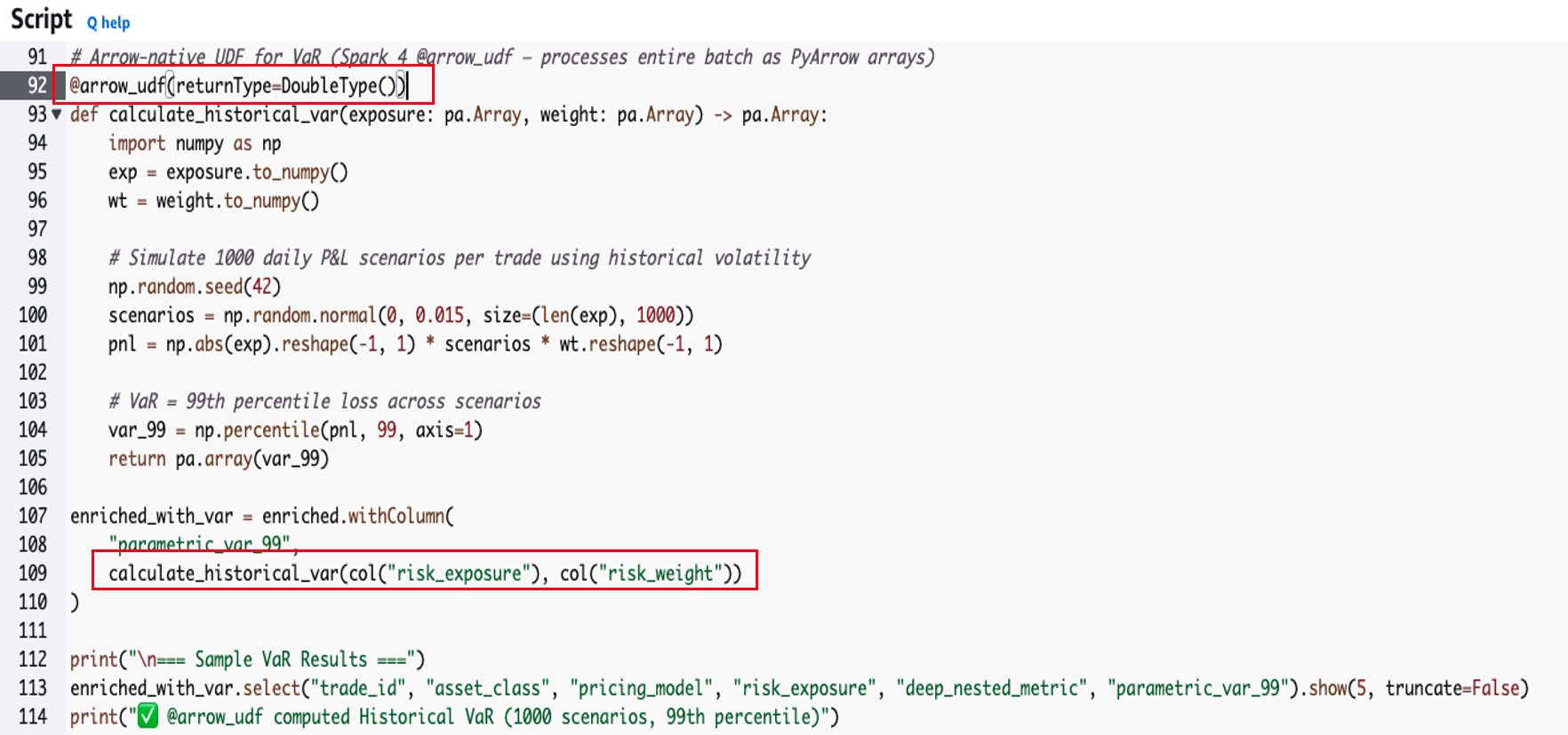
Figure 9: Arrow-native UDF computing Historical VaR

The @arrow_udf decorator is new in Spark 4.1. Your function receives and returns pyarrow.Array directly, operating on the entire batch of rows at once. There is no pickle serialization, no row-by-row invocation, and no Pandas conversion. Data flows as native Arrow columnar arrays between the JVM and Python. For compute-heavy operations like VaR across hundreds of thousands of rows, this can be significantly faster than traditional scalar UDFs. Additionally, you can use the built-in UDF profilers to identify performance and memory bottlenecks in compute-heavy UDFs such as VaR calculations.

Handle late trade corrections with deletion vectors

In financial markets, trade amendments and cancellations are common. The batch VaR job demonstrates this after completing the risk computation. It amends one trade and cancels another.

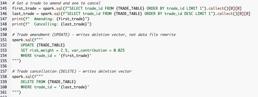
Figure 10: Amending and cancelling trades with merge-on-read

Prior to Iceberg v3, row-level deletes required either rewriting entire data files (copy-on-write) or maintaining separate positional delete files that store (file_path, row_position) pairs as Parquet rows (merge-on-read). Both approaches are expensive at scale. Copy-on-write rewrites gigabytes for a single amendment, and positional deletes degrade read performance as delete files accumulate (each read must parse and hash-join all delete records against the data file).

Because we configured the table with write.delete.mode='merge-on-read', UPDATEs and DELETEs write deletion vectors instead of positional delete files used in Iceberg v2. A deletion vector is a Roaring Bitmap stored in a Puffin file (.puffin), one per affected data file, marking which row positions are deleted. At read time, the engine loads a single bitmap and skips flagged positions with a bit check. No file joins, no linear scan through multiple delete files. The bitmap is compact regardless of how many rows are deleted, and read performance remains predictable as amendments accumulate.

The batch job also verifies the deletion vectors were created. You can see the results in the job’s output logs.

Figure 11: Output verifying deletion vectors were created

Clean up

To avoid incurring further charges, delete the CloudFormation stack. This removes all resources provisioned as part of this post, including the S3 bucket, Glue jobs, Iceberg tables, MSK cluster, and IAM roles.

Conclusion

In this post, we built a multi-layer market risk pipeline using AWS Glue 6.0 (real-time alerting, near-real-time ingestion, and batch analytics):

• Spark Real-Time Mode (RTM) on the real-time path delivers sub-second trade scoring and breach alerting, eliminating the micro-batch boundary so position limits are enforced before the next trade executes.
• Iceberg v3 Variant on the near-real-time path stores heterogeneous pricing vectors without schema flattening. One table handles equities, FX, and rates with different schemas per row.
• Variant shredding delivers faster reads by automatically extracting fields into separate typed Parquet columns at write time with no manual tuning required.
• Arrow-native UDFs eliminate pickle serialization overhead for Python-based risk calculations, processing data as vectorized columnar batches on the batch layer.
• Deletion vectors handle trade amendments and cancellations without costly data file rewrites, using compact Roaring Bitmaps instead of accumulating positional delete files.
• Default values reduce boilerplate in ingestion code.

To get started with AWS Glue 6.0, see the AWS Glue documentation. For more information about Apache Iceberg v3, see the Iceberg specification.

About the authors