Artificial Intelligence
Developing a business strategy by combining machine learning with sensitivity analysis
Machine learning (ML) is routinely used by countless businesses to assist with decision making. In most cases, however, the predictions and business decisions made by ML systems still require the intuition of human users to make judgment calls.
In this post, I show how to combine ML with sensitivity analysis to develop a data-driven business strategy. This post focuses on customer churn (that is, the defection of customers to competitors), while covering problems that often arise when using ML-based analysis. These problems include difficulties with handling incomplete and unbalanced data, deriving strategic options, and quantitatively evaluating the potential impact of those options.
Specifically, I use ML to identify customers who are likely to churn and then use feature importance combined with scenario analysis to derive quantitative and qualitative recommendations. The results can then be used by an organization to make proper strategic and tactical decisions to reduce future churn. This use case illustrates several common issues that arise in the practice of data science, such as:
- A low signal-to-noise ratio and a lack of clear correlation between features and churn rates
- Highly imbalanced datasets (wherein 90% of customers in the dataset do not churn)
- Using probabilistic prediction and adjustment to identify a decision-making mechanism that minimizes the risk of over-investing in churn issues
End-to-end implementation code is available in Amazon SageMaker and as a standalone on Amazon EC2.
In this use case, I consider a fictional company that provides different types of products. I will call its two key offerings products A and B. I only have partial information about the company’s products and customers. The company has recently seen an increase in customer defection to competitors, also known as churn. The dataset contains information on the diverse attributes of thousands of customers, collected and sorted over several months. Some of these customers have churned, and some have not. Using the list of specific customers, I will predict the probability that any one individual will churn. During this process, I attempt to answer several questions: Can we create a reliable predictive model of customer churn? What variables might explain a customer’s likelihood of churning? What strategies can the company implement to decrease churn?
This post will address the following steps for using ML models to create churn reduction strategies:
Exploring data and engineering new features
I first cover how to explore customer data by looking at simple correlations and associations between individual input features and the churn label. I also examine the associations (called cross-correlations, or covariances) between the features themselves. This allows me to make algorithmic decisions—notably, deciding which features to derive, change, or delete.
Developing an ensemble of ML models
Then, I build several ML algorithms, including automatic feature selection, and combine multiple models to improve performance.
Evaluating and refining ML model performance
In the third section, I test the performance of the different models I have developed. From there, I identify a decision-making mechanism that minimizes the risk of overestimating the number of customers who will churn.
Applying ML models to business strategy design
Finally, in a fourth section, I use the ML results to understand the factors that impact customer churn, derive strategic options, and quantitatively evaluate the impact of those options on churn rates. I do so by performing a sensitivity analysis, where I modify some factors that can be controlled in real life (such as the discount rate) and predict the corresponding reduction in churn expected for different values of this control factor. All predictions will be carried out with the optimal ML model identified in section 3.
Exploring data and engineering new features
Critical issues that often present problems during ML model development include the presence of collinear and low-variance features in the input data, the presence of outliers, and missing data (missing features and missing values for some features). This section describes how to handle each of these issues in Python 3.4 using Amazon SageMaker. (I also evaluated the standalone code on an Amazon EC2 instance with a Deep Learning AMI. Both are available.)
This kind of timestamped data can contain important patterns within certain metrics. I aggregated these metrics into daily, weekly, and monthly segments, which allowed me to develop new features to account for the metrics’ dynamic nature. (See the accompanying notebook for details.)
I then look at simple one-to-one (a.k.a. marginal) correlation and association measures between each individual feature, both original and new. I also look at the correlations between the features and the churn label. (See the following diagrams).
Low-variance features, features that do not change significantly when the churn label changes, can be handled by using marginal correlation and Hamming/Jaccard distances, as depicted in the following table. Hamming/Jaccard distances are measures of similarity designed specifically for binary outcomes. These measures provide perspective on the degree to which each feature might be indicative of churn.
It’s good practice to remove low-variance features as they tend not to change significantly no matter what you’re trying to predict. Consequently, their presence is unlikely to help your analysis and can actually make the learning process less efficient.
The following table shows the top correlations and binary dissimilarities between features and churn. Only the top features are shown out of 48 original and derived features. The Filtered column contains the results that I obtained when I filtered the data for outliers and missing values.
| Pearson correlations with churn | ||
| Feature | Original | Filtered |
| Margins | 0.06 | 0.1 |
| Forecasted product A | 0.03 | 0.04 |
| Prices | 0.03 | 0.04 |
| $value of discount | 0.01 | 0.01 |
| Current subscription | 0.01 | 0.03 |
| Forecasted product B | 0.01 | 0.01 |
| Number of products | -0.02 | -0.02 |
| Customer loyalty | -0.07 | -0.07 |
| Binary dissimilarities with churn | ||
| Feature | Hamming | Jaccard |
| Sales channel 1 | 0.15 | 0.97 |
| Sales channel 2 | 0.21 | 0.96 |
| Sales channel 3 | 0.45 | 0.89 |
The key takeaways from the preceding table are that three sales channels seem inversely correlated to churn and that most marginal correlations with churn are very small (≤ 0.1). Applying filters for outliers and missing values leads to marginal correlations with improved statistical significance. The right column of the preceding table depicts this effect.
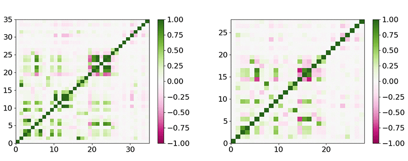
The issue of collinear features can be addressed by computing the covariance matrix between all features, as shown in the following diagram. This matrix provides new perspective on the amount of redundancy some features might have. It’s a good practice to remove redundant features because they create biases and demand more computation, again making the learning process less efficient.
The left graph in the preceding diagram indicates that some features, such as prices and some forecasted metrics, are collinear, with ρ > 0.95. I kept only one of each when I designed the ML models that I describe in the next section, which left me with about 40 features, as the right graph in the preceding diagram shows.
The issues of missing and outlier data are often handled by instituting empirical rules, such as deleting observations (customers) when some of their recorded data values are missing, or when they exceed three times the standard deviation across the sample.
Because missing data is a frequent concern, you can impute a missing value with the mean or median across the sample or population as an alternative to deleting observations. That’s what I did here: I replaced missing values with the median for each feature—except for features where more than 40% of data was missing, in which case I deleted the entire feature. The reader should note that a more advanced, best practice approach to imputing missing data is to train a supervised learning model to impute based on other features, but this can require a very large amount of effort so I do not cover it here. When I encountered outliers in the data, I deleted the customers with values beyond six standard deviations from the mean. In total, I deleted 140 out of 16096 (< 1%) observations.
Developing an ensemble of ML models
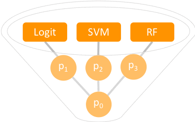
In this section, I develop and combine multiple ML models to harness the power of multiple ML algorithms. Ensemble modeling also makes it possible to use information from the entire dataset, even though the distribution of the churn label is highly unbalanced, as shown in the following flowchart.

Predicted probability
p0 = (p1 + p2 + p3) / 3
As it’s good practice to remove low-variance features, I further restricted the feature space to the most important features by applying a quick and simple variance filter. This filter removes features that display no variance for more than 95% of customers. To filter features based on their combined effects on customer churn, as opposed to their marginal effects, I carried out an ML-based feature selection using a grid search with stepwise regression. See details in the next section.
Before implementing the ML models, I randomly split the data into two groups, holding out a 30% test set. As discussed in the next section, I also used a 10-fold cross-validation on top of the 70%/30% split. K-folding is an iterative cycle that averages the performance over K evaluations, each testing on a separate K% holdout set of the data.
Three ML algorithms—logistic regression, support vector machine, and random forest—were trained separately, then combined in an ensemble, as depicted in the preceding flowchart. The ensemble approach is referred to as soft-voting in the literature because it takes the average probability of the different models and uses it to classify customer churn (also visible in the preceding flowchart).
Customers with churn represent only 10% of the data; therefore, the dataset is unbalanced. I tested two approaches to deal with class imbalance.
- In the first, simplest approach, the training is based on a random sampling of the abundant class (customers who didn’t churn) to match the size of the rare class (customers who did).
- In the second approach (shown in the following chart), I based the training on an ensemble of nine models using nine random samples of the abundant class (without replacement) and a full sample of the rare class for each model. I chose a 9-fold because the class imbalance is approximately 1-to-9 (as shown in the histogram in the following diagram). Therefore, 1-9 is the amount of sampling required to use all or nearly all of the data in the abundant class. This approach is more complex, but it uses all available information, improving generalization. I evaluate its effectiveness in the following section.

For both approaches, the performance is evaluated on a test set wherein class imbalance is maintained to account for real-world circumstances.
Evaluating and refining ML model performance
In this section, I test the performance of the different models I developed in the previous section. I then identify a decision-making mechanism that minimizes the risk of overestimating the number of customers who might churn (called the false positive rate).
The so-called receiver-operator characteristic (ROC) curve is often used in ML performance evaluation to complement contingency tables. The ROC curve provides an invariant measure of accuracy when changing the probability threshold to infer positive and negative classes (in this project, churn and no churn, respectively). It involves plotting all accurate positive predictions (true positives) against false positives, also known as fall out. See the following table.
The probabilities predicted by the different ML models are by default calibrated so that values where p > 0.5 correspond to one class and values where p < 0.5 correspond to the other class. This threshold is a hyperparameter that can be fine-tuned to minimize misclassified instances of one class. This is at the expense of increasing misclassification in the other, which can affect the accuracy and precision of different performance measures. In contrast, the area under the ROC curve is an invariant measure of performance—it remains the same for any threshold.
The following table depicts the performance of different ML models with a random sampling of the rare class (baseline) and the 9-fold ensemble of learners. You can see that the random forest has the best performance, and further that the 9-fold ensemble is better at generalizing, with an ROC AUC score of 0.68. This model is the best performer.
| Performance measures | ||||
| Algorithm | Accuracy | Brier | ROC | |
| Logit | 56% | 0.24 | 0.64 | |
| Stepwise | 56% | 0.24 | 0.64 | |
| SVM | 57% | 0.24 | 0.63 | |
| RF | 65% | 0.24 | 0.67 | |
| Ensemble | 61% | 0.23 | 0.66 | |
| 9-Logit Ensemble | 55% | 0.26 | 0.64 | |
| 9-SVM Ensemble | 61% | 0.25 | 0.63 | |
| 9-RF Ensemble | 70% | 0.24 | 0.68 | |
| 9-Ensemble Ensemble | 61% | 0.25 | 0.65 | |
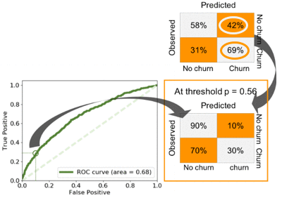
The following chart depicts the performance of the overall best learner (the 9-fold ensemble of random forest learners) and the optimization for precision and fall out. When using a probability threshold of 0.5, the best performer can predict 69% of the customers who might churn though with significant fall out of 42%.

Looking at the ROC curve, you can see that the same model can predict 30% of customers who will churn, with fall out minimized at 10%. Using a grid search, I found that the threshold is p = 0.56. If you want to minimize the risk of overestimating the number of customers who will churn (for example, because the attempts we make to keep those customers could be expensive), this is the model you might want to use.
Applying ML models to business strategy design
In this section, I use the ML models that I have developed to better understand the factors that impact customer churn, to derive strategic options for decreasing churn, and to evaluate the quantitative impact that deploying those options might have on churn rates.
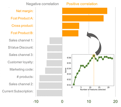
I used a stepwise logistic regression to assess the importance of features while taking into account their combined effect on churn. As shown in the following graph, the regression identifies 12 key features. The prediction score is highest when I include these 12 features in the regression model.
Among these 12 factors, the net margin, the forecasted purchase of products A and B, and the index that indicates multiple-product customers are the features that have the greatest tendency to induce churn. The factors that tended to reduce churn included three sales channels, one marketing campaign, the value of the discount, overall subscriptions, the loyalty of the customer, and the overall number of products purchased.

Therefore, providing a discount to customers with the highest propensity to churn seems to be a simple and effective strategy. Other strategic levers have also been identified, including boosting synergy between products other than A and B, sales channels 1–3, the marketing campaign, and long-term contracts. According to the data, pulling these levers is likely to decrease customer churn.
Finally, I used a sensitivity analysis: I applied a discount of up to 40% to customers that the ML model identified as likely to churn, then re-ran the model to evaluate how many customers were still predicted to churn after incorporating the discount.
When I set the model at a p threshold of 0.6 to minimize fall out to 10%, my analysis predicts that a 20% discount reduces churn by 25%. Given that the true positive rate at this threshold is about 30%, this analysis indicates that a 20% discount approach could eliminate at least 8% of churn. See the following graph for details. The discount strategy is a simple first step that an organization experiencing customer churn might consider taking to mitigate the issue.

Conclusion
In this post, I demonstrated how to do the following:
- Explore data and derive new features in order to minimize issues stemming from missing data and a low signal-to-noise ratio.
- Design an ensemble of ML models to handle strongly unbalanced datasets.
- Select the best-performing models and refine the decision threshold to maximize precision and minimize fall out.
- Use the results to derive strategic options and quantitatively assess their impact on churn rates.
In this particular use case, I developed a model that can identify 30% of customers who are likely to churn while limiting fall out to 10%. This study supports the efficacy of deploying a short-term tactic of offering discounts and instituting a long-term strategy based on building synergy between services and sales channels to retain more customers.
If you would like to run the code that produce the data and insights described in this blog post, just download the notebook and associated data file, then run each each cell one at a time.
About the author
 Jeremy David Curuksu is a data scientist and consultant in AI-ML at the Amazon Machine Learning Solutions Lab (AWS). He holds a MSc and a PhD in applied mathematics, and was a research scientist at EPFL (Switzerland) and MIT (US). He is the author of multiple scientific peer-reviewed articles and the book Data Driven which introduces management consulting in the new age of data science.