Use the built-in Amazon SageMaker Random Cut Forest algorithm for anomaly detection

Today, we are launching support for Random Cut Forest (RCF) as the latest built-in algorithm for Amazon SageMaker. RCF is an unsupervised learning algorithm for detecting anomalous data points or outliers within a dataset. This blog post introduces the anomaly detection problem, describes the Amazon SageMaker RCF algorithm, and demonstrates the use of the Amazon SageMaker RCF on an example real-world dataset.

Anomaly detection is critical

Suppose you have collected data on traffic volume over a period of time across multiple city blocks. Can you predict if a spike in traffic volume represents a collision or just the usual rush hour? Does it matter if the spike occurred at one block or several? Or suppose you have streams of network traffic between servers in a cluster. Can you automatically detect if the infrastructure is under a distributed denial of service (DDOS) attack or if the increase in network activity is benign?

An anomaly is an observation that diverges from otherwise well-structured or patterned data. For example, anomalies can manifest as unexpected spikes in time series data, breaks in periodicity, or unclassifiable data points. The inclusion of such anomalies in a dataset may drastically increase the complexity of a machine learning task since the “regular” data can often be described with a simple model.

The Amazon SageMaker Random Cut Forest algorithm

The Amazon SageMaker Random Cut Forest (RCF) algorithm is an unsupervised algorithm for detecting anomalous data points within a dataset. In particular, the RCF algorithm in Amazon SageMaker associates an anomaly score with each data point. An anomaly score with low values indicates that the data point is considered “normal” whereas high values indicate the presence of an anomaly. The definitions of “low” and “high” depend on the application, but common practice suggests that scores beyond three standard deviations from the mean score are considered anomalous.

The RCF algorithm in Amazon SageMaker works by first obtaining a random sample of the training data. Since the training data may be too large to fit on one machine, a technique called reservoir sampling is used to efficiently draw the sample from a stream of data. Subsamples are then distributed to each constituent tree in the random cut forest. Each subsample is organized into a binary tree by randomly subdividing bounding boxes until each leaf represents a bounding box containing a single data point. The anomaly score assigned to an input data point is inversely proportional to its average depth across the forest. For more information see the SageMaker RCF documentation page. The underlying algorithm is based on the work described in the references section at the end of this blog post.

Hands-on example: Detecting events in New York City from taxi ridership data

We demonstrate the Amazon SageMaker RCF on an example dataset consisting of six months of taxi ridership volume in New York City. These data are publicly available in the Numenta Anomaly Benchmark (NAB) New York City Taxi dataset. In the code examples that follow, we train a SageMaker RCF model and use the model to detect anomalies in the ridership data. See the introductory notebook for more information.

Obtain, inspect, and store data in Amazon S3

First, we obtain and plot the NAB dataset. These data span approximately six months of taxi ridership in New York City where each data point represents a 30-minute window of ridership volume.

import pandas
import urllib.request

data_filename = 'nyc_taxi.csv'
data_source = 'https://raw.githubusercontent.com/numenta/NAB/master/data/realKnownCause/nyc_taxi.csv'

urllib.request.urlretrieve(data_source, data_filename)
taxi_data = pandas.read_csv(data_filename, delimiter=',')
taxi_data.plot(title='Taxi Ridership in NYC')

As we expect, taxi ridership is approximately periodic: during the day traffic volume is high, especially during usual commute times, and it’s low in the middle of the night. We also observe the weekly periodicity where ridership is higher on work days than during the weekend. By taking a closer look at the plot, we can easily observe several anomalous data points. After all, human beings are highly visual creatures, and we have developed excellent pattern-detection capabilities over the course of millions of years of evolution. In particular, these anomalies occur in places where ridership spikes, dips, or breaks the characteristic periodic behavior. Some of these correspond to known events, such as the New York City Marathon at t=5954, New Year’s Eve at t=8833, and a major snow storm at t=10090.

Like many other Amazon SageMaker algorithms, training works best with data encoded in RecordIO Protobuf format. Below, we convert the CSV-formatted data and push the data to our Amazon S3 bucket.

def convert_and_upload_training_data(
    ndarray, bucket, prefix, filename='data.pbr'):
    import boto3
    import os
    from sagemaker.amazon.common import numpy_to_record_serializer

    # convert Numpy array to Protobuf RecordIO format
    serializer = numpy_to_record_serializer()
    buffer = serializer(ndarray)

    # upload to S3
    s3_object = os.path.join(prefix, 'train', filename)
    boto3.Session().resource('s3').Bucket(bucket).Object(s3_object).upload_fileobj(buffer)
    s3_path = 's3://{}/{}'.format(bucket, s3_object)
    return s3_path

bucket = '<my-s3-bucket>' # <-- use your own bucket, here
prefix = 'sagemaker/randomcutforest'
s3_train_data = convert_and_upload_training_data(
    taxi_data.value.as_matrix().reshape(-1,1),
    bucket,
    prefix)

Training the model

Before training a SageMaker Random Cut Forest model on this dataset, we must first specify training job parameters such as the Amazon Elastic Container Registry (ECR) Docker container for the Amazon SageMaker Random Cut Forest algorithm, the location of the training data, and the instance type on which we will run the algorithm. We also specify algorithm-specific hyperparameters. The two primary hyperparameters available in the Amazon SageMaker RCF algorithm are num_trees and num_samples_per_tree.

The hyperparameter, num_trees, sets the number of trees used in the RCF model. Each tree learns a separate model from a subsample of the input training data and outputs an anomaly score for a given data point inversely proportional to its depth within the tree. The anomaly score assigned to a data point by the entire RCF model is equal to the average score reported, calculated by the constituent trees. The hyperparameter, num_samples_per_tree, dictates how many randomly sampled training data points are sent to each tree. A good choice for num_samples_per_tree is such that its inverse approximates the expected percentage of anomalies in the dataset. See Amazon SageMaker RCF – How it Works for more information.

The following code fits the SageMaker RCF model to the taxi data using 50 trees and sending 200 data points to each tree.

import boto3
import sagemaker

containers = {
    'us-west-2': '174872318107.dkr.ecr.us-west-2.amazonaws.com/randomcutforest:latest',
    'us-east-1': '382416733822.dkr.ecr.us-east-1.amazonaws.com/randomcutforest:latest',
    'us-east-2': '404615174143.dkr.ecr.us-east-2.amazonaws.com/randomcutforest:latest',
    'eu-west-1': '438346466558.dkr.ecr.eu-west-1.amazonaws.com/randomcutforest:latest'}
region_name = boto3.Session().region_name
container = containers[region_name]

session = sagemaker.Session()

rcf = sagemaker.estimator.Estimator(
    container,
    sagemaker.get_execution_role(),
    output_path='s3://{}/{}/output'.format(bucket, prefix),
    train_instance_count=1,
    train_instance_type='ml.c5.xlarge',
    sagemaker_session=session)

rcf.set_hyperparameters(
    num_samples_per_tree=200,
    num_trees=50,
    feature_size=1)

s3_train_input = sagemaker.session.s3_input(
    s3_train_data,
    distribution='ShardedByS3Key',
    content_type='application/x-recordio-protobuf')

rcf.fit({'train': s3_train_input})

Predicting anomaly scores

We now use this trained model to compute anomaly scores for each of the training data points. As with other Amazon SageMaker algorithms, we begin by creating an inference endpoint using the model generated earlier.

from sagemaker.predictor import csv_serializer, json_deserializer

rcf_inference = rcf.deploy(
    initial_instance_count=1,
    instance_type='ml.c5.xlarge',
)

rcf_inference.content_type = 'text/csv'
rcf_inference.serializer = csv_serializer
rcf_inference.deserializer = json_deserializer

Next, we run inference on the entire training set, obtaining the anomaly score associated with each point. We use a simple, standard technique for classifying anomalies: all anomaly scores outside three standard deviations from the mean score are considered anomalous. More robust techniques exist, but this method is sufficient for this demonstration.

results = rcf_inference.predict(taxi_data.value.as_matrix().reshape(-1,1))
scores = [datum['score'] for datum in results['scores']]
taxi_data['score'] = pandas.Series(scores, index=taxi_data.index)

score_mean = taxi_data.score.mean()
score_std = taxi_data.score.std()

score_cutoff = score_mean + 3*score_std
anomalies = taxi_data[taxi_data['score'] > score_cutoff]

Finally, we plot the scores along with the taxi ridership data, highlighting the data points that are considered anomalous.

import matplotlib.pyplot as plt

fig, ax1 = plt.subplots()
ax2 = ax1.twinx()

ax1.plot(taxi_data['value'], alpha=0.8)
ax1.set_ylabel('Taxi Ridership', color='C0')
ax1.tick_params('y', colors='C0')

ax2.plot(taxi_data['score'], color='C1')
ax2.plot(anomalies.index, anomalies.score, 'ko')
ax2.set_ylabel('Anomaly Score', color='C1')
ax2.tick_params('y', colors='C1')

fig.suptitle('Taxi Ridership in NYC')
plt.show()

We see in the above plot that the SageMaker RCF algorithm indeed catches some of the known anomalies: the New York City Marathon at t=5954, New Year’s Eve at t=8833, and a snow storm at t=10090. Due to the small number of available data points, however, we pick up some noise in our anomaly score predictions as a result of the model’s proclivity toward identifying fine-grained changes in time series behavior.

Pre-processing strategies: Improving accuracy with shingling

In many machine learning tasks, it’s common to pre-process the data in order to improve accuracy and performance. In anomaly detection algorithms, shingling is a standard technique that turns one-dimensional data into s-dimensional data by converting contiguous subsequences of length s into s-dimensional vectors. The benefit is the ability to better detect breaks in periodicity as well as to filter out small-scale noise in the original anomaly scores. Note that if the shingle size is too small, then the random cut forest is more sensitive to small fluctuations in the data, as seen in the ridership plots earlier in this blog post. However, if the shingle size is too large, then smaller scale anomalies might be lost. Like the SageMaker RCF hyperparameters, num_trees and num_samples_per_tree, optimal values for shingle size are problem-dependent.

The diagram that follows illustrates a shingling transformation of a one-dimensional data stream into four-dimensional shingles. Note that the first shingled data point consists of the first four data points, in order, the second shingled data point consists of the next four, and so on.

Each data point in the NYC taxi data represents a 30-minute period of ridership. It’s reasonable to expect that ridership is periodic each day: on a normal day the ridership is more or less the same. So, on Monday, ridership is the same as it is on Tuesday. Therefore, it makes sense to shingle our data with shingle size of 48. (24 hours = 48 data points * 0.5 hours per data point.) We use the following function to shingle the NYC taxi data.

def shingle(data, shingle_size=48):
    import numpy as np
    num_data = len(data)
    shingled_data = np.zeros((num_data-shingle_size, shingle_size))
    
    for n in range(num_data - shingle_size):
        shingled_data[n] = data[n:(n+shingle_size)]
    return shingled_data

In the following figure we plot the resulting anomaly scores after applying this transformation to the original dataset and running new training and inference jobs on Amazon SageMaker.

We see that the shingled approach does a better job identifying the large-scale anomalies such as the dramatic drops in ridership during the snow storm at t=10090. If you have a labeled test dataset, then SageMaker RCF can output a number of accuracy metrics such as precision, recall, and F1-score. By analyzing these metrics, you can determine optimal values for num_trees and num_samples_per_tree and maximize these accuracy scores.

Benchmarks

Amazon SageMaker RCF scales well with respect to number of features, dataset size, and number of instances. Later in this post, we present SageMaker RCF performance, accuracy, and scaling benchmarks. These benchmarks are performed on synthetic data sets consisting of two Gaussian-distributed data clusters representing the “normal” data and a small Gaussian-distributed cluster representing the “anomalous” data lying between the two normal clusters. Approximately 0.5% of each dataset consists of anomalous data points. Each experiment was run on an ml.m4.xlarge instance type.

Performance

We measured the performance of SageMaker RCF on datasets consisting of varying feature dimension and size. In the following graphic, we plot the total amount of time required to train an RCF model. In each experiment we use num_trees=100 and num_samples_per_tree=256. Note that training time scales linearly as a function of data set size.

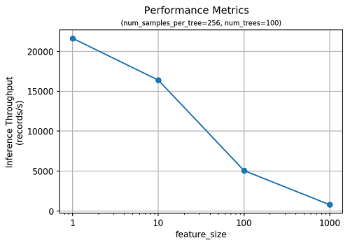
SageMaker RCF is also efficient at making anomaly predictions. In the following figure, we plot inference throughput as a function of feature dimension.

Accuracy

In the field of anomaly detection, several standard measurements are used to determine the accuracy of an anomaly detection algorithm. Precision is the ratio of correctly detected anomalies and number of points labeled anomalous by the algorithm. Recall is the ratio of correctly detected anomalies and total known anomalies. F1 is the harmonic mean of precision and recall. In the plot that follows, we present accuracy metrics on a 10-dimensional synthetic dataset with 100 million records as a function of the hyperparameter, num_samples_per_tree. As mentioned earlier, the inverse of num_samples_per_tree approximates the percentage of anomalies in the dataset.

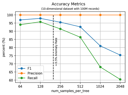
Note that we achieve maximum F1-score for values of num_samples_per_tree which correspond to the known percentage of anomalies in the synthetic dataset. We compared the accuracy of SageMaker RCF to Scikit-learn’s Isolation Forest (IF) algorithm. On small datasets, the two algorithms have comparable accuracy: on a 10-dimensional dataset with 10,000 records, both algorithms achieve an F1-score of 99.6%. However, Scikit-learn IF fails to run on any of the larger data sets used in our study.

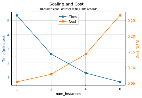
Scaling

SageMaker RCF scales nearly perfectly with the number of instances: twice as many instances approximately halves the amount of time needed to train a model.

Conclusion

Amazon SageMaker provides a fully managed, end-to-end solution to the problem of training and deploying large-scale machine learning models. The Amazon SageMaker RCF algorithm enables you to use Amazon SageMaker for anomaly detection. The example presented in this blog post uses a small, one-dimensional time series dataset. However, the algorithm is especially well-suited for performing anomaly detection with large-scale, large-dimensional data sets. The AWS AI Algorithms team looks forward to hearing about your innovative uses of the Amazon SageMaker RCF algorithm, as well as your suggestions on improvements.

References

[1] Sudipto Guha, Nina Mishra, Gourav Roy, and Okke Schrijvers. “Robust random cut forest based anomaly detection on streams.” In International Conference on Machine Learning, pp. 2712-2721. 2016.

[2] Byung-Hoon Park, George Ostrouchov, Nagiza F. Samatova, and Al Geist. “Reservoir-based random sampling with replacement from data stream.” In Proceedings of the 2004 SIAM International Conference on Data Mining, pp. 492-496. Society for Industrial and Applied Mathematics, 2004.

About the Authors

Chris Swierczewski is an Applied Scientist on the AWS AI Algorithms team, which is responsible for researching and developing the machine learning algorithms in Amazon SageMaker. Before Amazon, Chris was a Ph.D. student in Applied Mathematics at the University of Washington. He likes to go hiking, backpacking, and camping with his wife and their dog, River.

Julio Delgado Mangas is a Software Development Engineer on the AWS AI Algorithms team. He has contributed to AWS services like Amazon CloudWatch and the Amazon QuickSight SPICE engine. Before joining Amazon he was a research engineer on the Human Brain Project.

Madhav Jha is an Applied Scientist on the AWS AI Algorithms team where he uses his background in sublinear algorithms to develop scalable machine learning algorithms. He is a theoretical computer scientist who enjoys coding. He is always up for coffee conversations on startups and technology.

Luka Krajcar is a Software Development Engineer on the AWS AI Algorithms team. He received his M.S. in Computer Science at the Faculty of Electrical Engineering and Computing at the University of Zagreb. Outside of work, Luka enjoys reading fiction, running, and video gaming.