Using Spectrum fine-tuning to improve FM training efficiency on Amazon SageMaker AI

Optimizing generative AI applications relies on tailoring foundation models (FMs) using techniques such as prompt engineering, RAG, continued pre-training, and fine-tuning. Efficient fine-tuning is achieved by strategically managing hardware, training time, data volume, and model quality to reduce resource demands and maximize value.

Spectrum is a new approach designed to pinpoint the most informative layers within a foundation model (FM). Using this method, you can selectively fine-tune just a portion of the model, thereby enhancing training efficiency. Recently, several methods have been developed to fine-tune language models more efficiently, reducing both computational resources and time. One widely used technique is Quantized LoRA (QLoRA) which combines low rank adaptation (LoRA) with quantization of the original model for training. This method yields impressive outcomes, only slightly inferior to full fine-tuning, while using just a fraction of GPU resources. However, QLoRA applies low-rank adaptation uniformly throughout the entire model.

In this post you will learn how to use Spectrum to optimize resource use and shorten training times without sacrificing quality, as well as how to implement Spectrum fine-tuning with Amazon SageMaker AI training jobs. We will also discuss the tradeoff between QLoRA and Spectrum fine-tuning, showing that while QLoRA is more resource efficient, Spectrum results in higher performance overall.

How Spectrum fine-tuning works

Spectrum first evaluates the weight matrices across the layers of a FM and calculates a Signal-to-Noise Ratio (SNR) layer by layer. Instead of quantizing all layers, Spectrum selectively trains a subset of layers in full precision based on their SnR and freezes the rest of the model. You can also perform FP16, BF16, or FP8 training which is available in newer GPUs.

By leveraging Random Matrix Theory and the Marchenko-Pastur distribution, it effectively differentiates between signal and noise. Based on a configurable, predetermined percentage (for example, 30%), Spectrum identifies the most informative layers of each type (such as mlp.down_proj, and self_attn.o_proj) so you can freeze the rest of the model and focus fine-tuning on those selected layers.

Solution overview

In this example, you will learn how to use Spectrum along with Amazon SageMaker AI fully managed training jobs to fine-tune a Qwen3-8B model. Spectrum fine-tuning involves a few key steps. First, Spectrum will download the desired model to be analyzed (automatically using AutoModelforCausalLM). Then, it will run an analysis to determine the Signal-to-Noise Ratio (SNR) for each layer in the model. Based on this analysis, Spectrum will create a file specifying a subset of layers based on the chosen percentage that can be used as input to the training job. Next, you can use the training script provided in this example or implement the sample code into your own that can process the Spectrum output and selectively freeze or unfreeze layers accordingly. Finally, you will create an Amazon SageMaker AI training job, providing the Spectrum analysis as an input. The goal of this process is to leverage Spectrum’s insights about the model layers to fine-tune the model more effectively, by focusing the training on the most relevant layers. A complete sample can be found in the SageMaker Distributed Training GitHub repository.

Prerequisites

Before starting this tutorial, verify you have:

• An AWS account with permissions to create SageMaker resources. For setup instructions, see Set up an AWS account and create an administrator user.
• Set up Amazon SageMaker Studio to run the JupyterLab notebook code.
  • If using a SageMaker Studio space for this example, it is advised to use a ml.m5.16xlarge instance with at least 50GB of disk space to download models and perform analysis quickly.
• Open terminal and git clone https://github.com/aws-samples/amazon-sagemaker-generativeai then go to folder  3_distributed_training/spectrum_finetuning/ to run this spectrum_training notebook.

The solution consists of two steps:

1. Cloning the Spectrum repository, then running the analysis scripts to identify the most influential layers and generate an output file to use in model training.
2. Supplying the Spectrum output along with training data to a fully managed SageMaker training job to fine-tune the model by running the Juypter notebook from the sample repository.

Performing Spectrum analysis

Go to the notebook and run below cell to download latest download the latest Spectrum release from the  QuixiAI Spectrum GitHub repository:

spectrum_clone_folder = "~/spectrum"
!git clone https://github.com/QuixiAI/spectrum.git {spectrum_clone_folder}

After cloning the repository, you can invoke Spectrum to run the model analysis. In this step, Spectrum will analyze the Signal-to-Noise Ratio (SNR) of the various low-level layers in your model. From there, it will rank them and allow you to select a percentage of the most influential layers to use in model training.

To generate the configuration, run the following command, supplying a HuggingFace Model ID and the percentage of layers you intend to unfreeze. By default, the entire model is frozen, and this percentage specifies how many layers will be made trainable by unfreezing. A smaller percentage of unfrozen layers leads to lower memory usage, but the optimal balance between the percentage of unfrozen layers and training/model performance will depend on your specific use case.

Note: Spectrum’s UI is interactive and cannot be run inside of this notebook. Please run the following cell, execute it in your terminal, then resume notebook execution. There is nothing from the terminal that you need to copy over.

The following cell generates a shell command that you need to run in your terminal

python3 spectrum.py --model-name <HF_MODEL_ID> --top-percent <PCT_LAYERS_TO_TRAIN>

In this example, to process Qwen3-8B at with 25% unfrozen layers, enter the following command into your environment’s terminal. This cannot be run in a Jupyter cell because it is an interactive shell:

cd Spectrum
python3 spectrum.py --model-name Qwen/Qwen3-8B --top-percent 25

You’ll then be prompted for a batch size value for the analysis as shown in the image below. You will see batch size 16 and click “OK” to proceed with download.

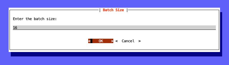
This example was created with a batch size of 16. Larger batch sizes allow for better calculation of the SNR gradients, due to being able to average across more samples. Too small of a batch size will result in more variance, introducing more “noise” into the SNR distribution, potentially leading to poor results. However, too large of a batch size will result in “oversampling” where the signal is lost in too many samples. Larger batch sizes will also require more resources for processing.

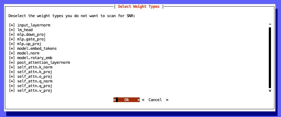
After model download and initial processing is completed, you’ll decide the layer types to include in your analysis. Deselect any that you don’t want to include. If you aren’t sure how to best optimize your model, it is recommended to select every layer type as shown in the image below and click “OK” to continue.

The underlying principles of spectrum fine-tuning, which involve selectively training layers based on their signal-to-noise ratio, can be applied to vision models. Although spectrum was developed for language models, the core idea of efficiently fine-tuning by focusing on the most informative layers can be extended to vision transformers (ViTs) and other vision architectures.

If you’d like to select specific layer types, use the following as a reference:

• Attention layers are critical for capturing contextual relationships between tokens and play a significant role in how the model understands and generates language. Selecting these for fine-tuning helps improve the model’s ability to focus on relevant parts of the input sequence for a given task.
• MLP layers (Multi-Layer Perceptrons) are responsible for transforming the token representations and contribute to the model’s capacity to learn and store factual knowledge. Fine-tuning them can enhance the model’s understanding of domain-specific vocabulary and concepts relevant to your fine-tuning task.
• Embedding layers are responsible for transforming categorical data (like tokens) into numerical vectors the model can process. Fine-tuning these layers might be beneficial if your target dataset involves a significantly different vocabulary or domain compared to the pre-training data.

The analysis job will output 3 files:

• A complete SNR breakdown of the analyzed layers (model_snr_results/snr_results_Qwen-Qwen3-8B.json)

    "model.layers.35.input_layernorm": {
        "snr": 1.0,
        "type": "input_layernorm"
    },
    "lm_head": {
        "snr": 253.33468627929688,
        "type": "lm_head"
    },
    "model.layers.0.mlp.down_proj": {
        "snr": 0.5318950414657593,
        "type": "mlp.down_proj"
    },
    "model.layers.1.mlp.down_proj": {
        "snr": 0.08824645727872849,
        "type": "mlp.down_proj"
    },

• A file with the layers sorted and grouped by type (snr_results_Qwen-Qwen3-8B_sorted.json)

{
    "input_layernorm": {
        "model.layers.0.input_layernorm": 1.0,
        ...
    },
    "lm_head": {
        "lm_head": 253.33468627929688
    },
    "mlp.down_proj": {
        "model.layers.10.mlp.down_proj": 1.797685146331787,
        ...
    },
    "mlp.gate_proj": {
        "model.layers.34.mlp.gate_proj": 0.8340917825698853,
        ...
    },
    "mlp.up_proj": {
        "model.layers.9.mlp.up_proj": 2.655043601989746,
        ...
    },
    "model.embed_tokens": {
        "model.embed_tokens": 0.14815816283226013
    },
    ...
}

• A percentage-specific file with the layers that should remain unfrozen during training (snr_results_Qwen-Qwen3-8B_unfrozenparameters_25percent.yaml)

unfrozen_parameters:
- ^lm_head.weight$
- ^model.embed_tokens.weight$
# input_layernorm layers
- model.layers.0.input_layernorm
...
# lm_head layers
# mlp.down_proj layers
- model.layers.10.mlp.down_proj
...
# mlp.gate_proj layers
- model.layers.34.mlp.gate_proj
...
# mlp.up_proj layers
...
# model.embed_tokens layers
...

The first time an analysis is executed, the model artifacts are downloaded and fully analyzed, then later runs output the percentage specific file using the saved analysis.

When running analysis, it is important to provide enough local CPU/memory to load the model and process it in a timely fashion. Using GPU resources can make analysis even faster. In either scenario, the result can be saved and reused to avoid needing to re-run it for other projects. In this example, processing the spectrum layers on CPU using a ml.m5.16xlarge SageMaker Studio space took about 3-5 minutes.

Preparing for training

Next take the snr_results_Qwen-Qwen3-8B_unfrozenparameters_25percent.yaml and put it into the folder with your training script. This file will be created in the spectrum folder that you cloned earlier. If you are using the sample notebook, it will handle copying this for you by running below code in your notebook:

spectrum_output_filename = f"snr_results_{filesafe_model_id}_unfrozenparameters_{spectrum_layer_percent}percent.yaml"
spectrum_output_filepath = f"{spectrum_clone_folder}/{spectrum_output_filename}"
spectrum_output_filepath

We have already incorporated  below code in the training script for this notebook example for spectrum fine tuning. You can proceed with the notebook for next steps in the notebook.

In case you would want to deep dive how you can setup Spectrum fine tuning for your own scripts. This section outlines how you would setup Spectrum fine tuning in your own training script.

Use the following code in your training script to process the Spectrum output and freeze/unfreeze appropriate parameters. This will freeze the entire model, then unfreeze the layers present in the spectrum analysis file. This filename should be included as an environment variable in your training job, so the script can fetch the correct one.

def setup_model_for_spectrum(model, spectrum_config_path):
    unfrozen_parameters = []
    with open(spectrum_config_path, "r") as fin:
        yaml_parameters = fin.read()

    # get the unfrozen parameters from the yaml file
    for line in yaml_parameters.splitlines():
        if line.startswith("- "):
            unfrozen_parameters.append(line.split("- ")[1])

    # freeze all parameters
    for param in model.parameters():
        param.requires_grad = False
        
    # unfreeze Spectrum parameters
    for name, param in model.named_parameters():
        if any(
            re.match(unfrozen_param, name)
            for unfrozen_param in unfrozen_parameters
        ):
            param.requires_grad = True

    return model

Later in your training script, load the model  into memory and pass it to the setup_model_for_spectrum function to freeze/unfreeze layers based on your Spectrum config.

model = AutoModelForCausalLM.from_pretrained(
    script_args.model_id,
    trust_remote_code=True,
    #quantization_config=bnb_config,
    use_cache=not training_args.gradient_checkpointing,
    cache_dir="/tmp/.cache",
    **model_configs
)

if training_args.gradient_checkpointing:
        model.gradient_checkpointing_enable()
else:
    if training_args.gradient_checkpointing:
        model.gradient_checkpointing_enable(gradient_checkpointing_kwargs={"use_reentrant": False})

if script_args.spectrum_config_path:
    model = setup_model_for_spectrum(model, script_args.spectrum_config_path)

With your training script configured, you can incorporate it into a SageMaker managed training job using the Amazon SageMaker Python SDK ModelTrainer and the Amazon SageMaker managed PyTorch training container. The ModelTrainer class simplifies the experience of customizing your training job, allowing you to supply a custom training script via the entry_script param at initialization.

First, specify a basic configuration including the model_id, instance_type, and output_path for the final model, and a reference to the training container.

model_id = "Qwen/Qwen3-8B"
instance_type = "ml.p4d.24xlarge"
output_path = "s3://<your_s3_bucket>/models/"

# Find a PyTorch SageMaker managed training container
image_uri = sagemaker.image_uris.retrieve(
    framework="pytorch",
    region=sagemaker_session.boto_session.region_name,
    version="2.6.0",
    instance_type=instance_type,
    image_scope="training"
)

Next, configure your ModelTrainer instance. Specify the local location of your training code, the compute requirements for the training job, and other training job configuration options.

# define Training Job Name 
job_name = f"train-{model_id.split('/')[-1].replace('.', '-')}-sft-spectrum-{spectrum_layer_percent}-script"

# Define the script to be run
source_code = SourceCode(
    source_dir="./scripts",
    requirements="requirements.txt",
    entry_script="train_spectrum.py",
)

# Define the compute
compute_configs = Compute(
    instance_type=instance_type,
    instance_count=1,
)

# Define the ModelTrainer
model_trainer = ModelTrainer(
    training_image=image_uri,
    source_code=source_code,
    base_job_name=job_name,
    compute=compute_configs,
    distributed=Torchrun(),
    stopping_condition=StoppingCondition(
        max_runtime_in_seconds=36000
    ),
    hyperparameters={
        "config": "/opt/ml/input/data/config/args.yaml" # Path to model training configuration file
    },
    output_data_config=OutputDataConfig(
        s3_output_path=output_path
    )
)

Then, define your training job inputs for training, validation, and configuration data.

# Define training inputs

train_input = InputData(
    channel_name="train",
    data_source=train_dataset_s3_path, # S3 path where training data is stored
)

test_input = InputData(
    channel_name="test",
    data_source=test_dataset_s3_path, # S3 path where training data is stored
)

config_input = InputData(
    channel_name="config",
    data_source=train_config_s3_path, # S3 path where training data is stored
)

data = [train_input, test_input, config_input]

Finally, start the training job by running the following:

# Start training job
model_trainer.train(input_data_config=data, wait=True)

By using model_train.train(wait=true) in the previous function, you can view the training output logs live in the notebook or you can view the training logs in the console under training jobs. Amazon SageMaker AI training jobs are ephemeral, so you only pay for the time your job is running.

Clean up

If you would like to stop your training job before it completes, navigate to the Jobs section of the SageMaker Studio UI, select Training, then select your running job and choose Stop. To stop and delete the SageMaker Studio spaces, follow these clean up steps in the SageMaker Studio documentation. You must delete the S3 bucket and the hosted model endpoint to stop incurring costs. You can delete the real-time endpoints you created using the SageMaker console. For instructions, see Delete Endpoints and Resources.

Results

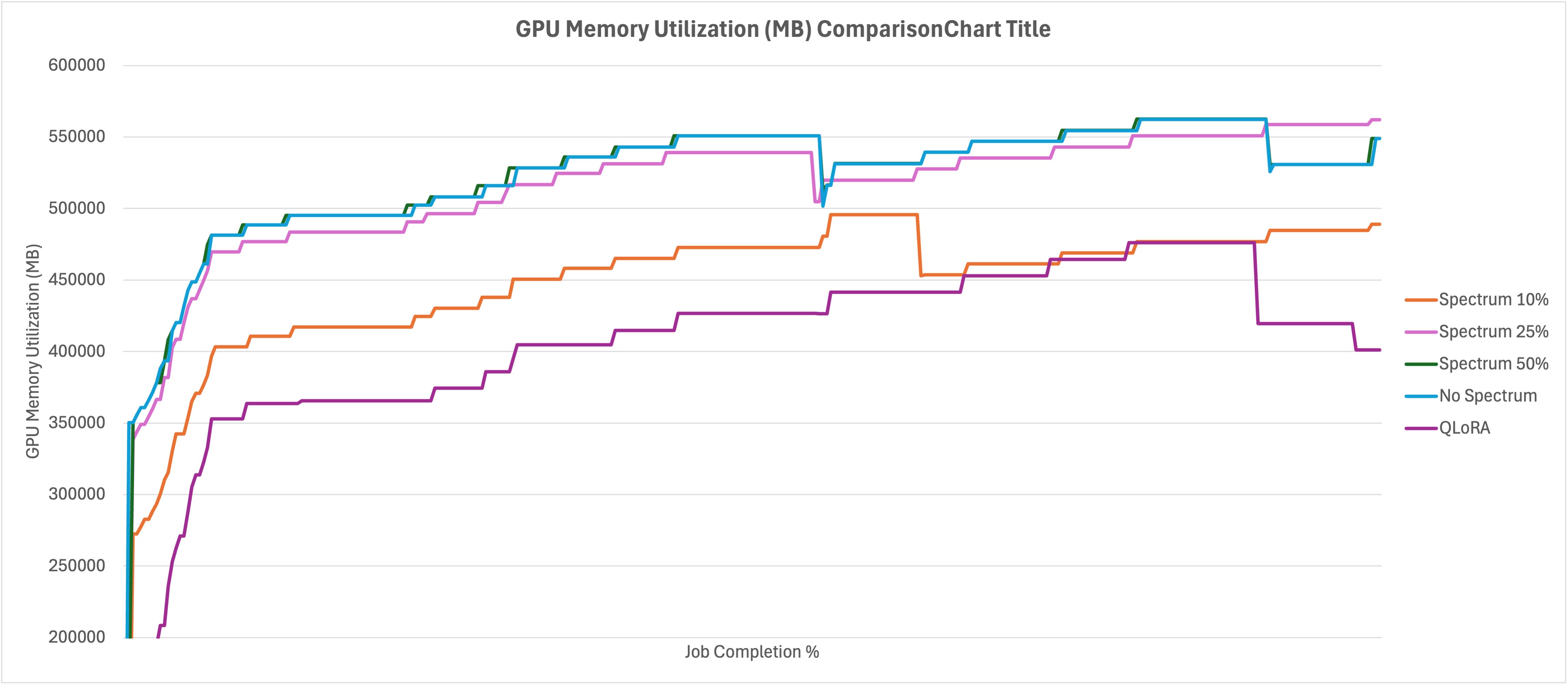
With the training job complete, it is time to look at the results. This example was run with Spectrum at 10, 25, and 50% as well as at full-parameters (no Spectrum) with the same training configuration (ml.p4de.24xlarge – NVIDIA A100, 640GB VRAM, 1152GiB RAM) with a batch size of 8. The the Stanford Question Answering Dataset (SQuAD) was used as training/validation data. To avoid CUDA Out-of-Memory issues, offload_params in the training job was set to true, allowing parameters to be offloaded to CPU memory in cases of insufficient GPU memory. This means that in order to understand complete memory utilization during the job, both memory metrics need to be inspected. This also affects training performance, but is a good simulation of a real-world use case where resources are limited.

Let’s look at the resource utilization first, then the impact of the different approaches on training validation loss. Starting with GPU Memory, in the graph below you can see that the 10% run easily fits within the memory footprint, while the 50% and no Spectrum runs start to hit a ceiling and offload layers to CPU memory. While we chose to keep everything consistent in this example, the 10% run could have benefitted further from an increased batch size. QLoRA is a clear winner here, using significantly less resources across the board, even compared to Spectrum 10%.

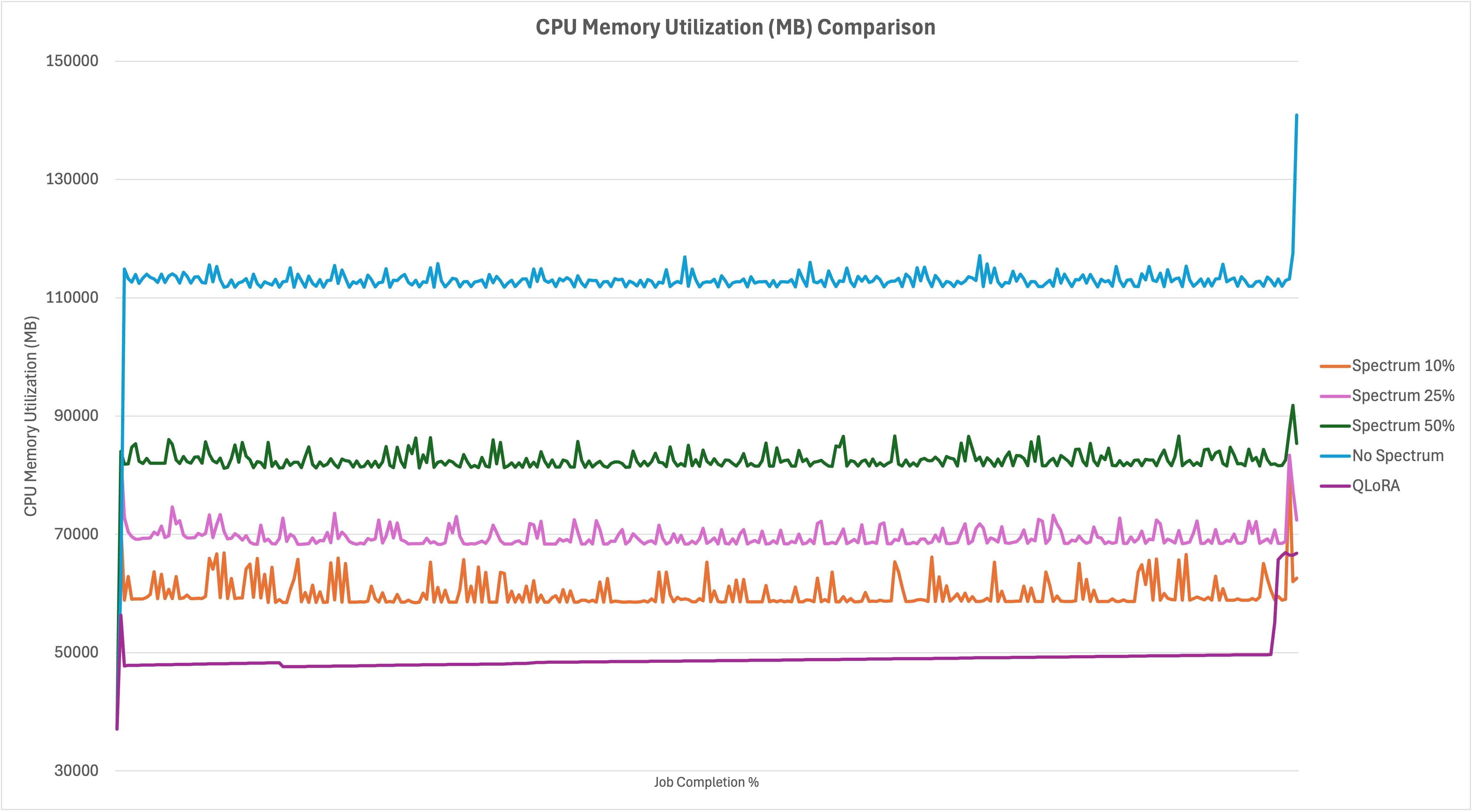
Looking at CPU Memory consumption comparison graph below, you can see where the offloading of parameters occurred in the different scenarios. The No Spectrum tuning example exhausted almost all of the available CPU memory near the end of the job, in addition to the GPU memory in the previous chart. Since the 10% run fit completely in GPU memory without offloading, the CPU memory consumption was minimal, while 25% and 50% used incrementally more. Again, QLoRA has the most efficient use of memory for the duration of the job. There is a large spike at the end of the run, related to merging the adapter back into the base model.

Comparing validation loss graph as shown below across the runs shows what you might already expect. The high number of parameters that needed to be influenced in the no Spectrum run starts the job off at a much higher loss than the Spectrum runs, but it eventually catches up over time. The No Spectrum run ends up with similar resulting loss metrics as 25% and 50% Spectrum runs, with 10% marginally higher. As efficient as QLoRA was in the resource utilization comparisons early, you can see that it comes at a large(relative) impact to validation loss. The other runs in this example surpassed the QLoRA training loss by the 10% job completion mark, then continued to improve as training time went on.

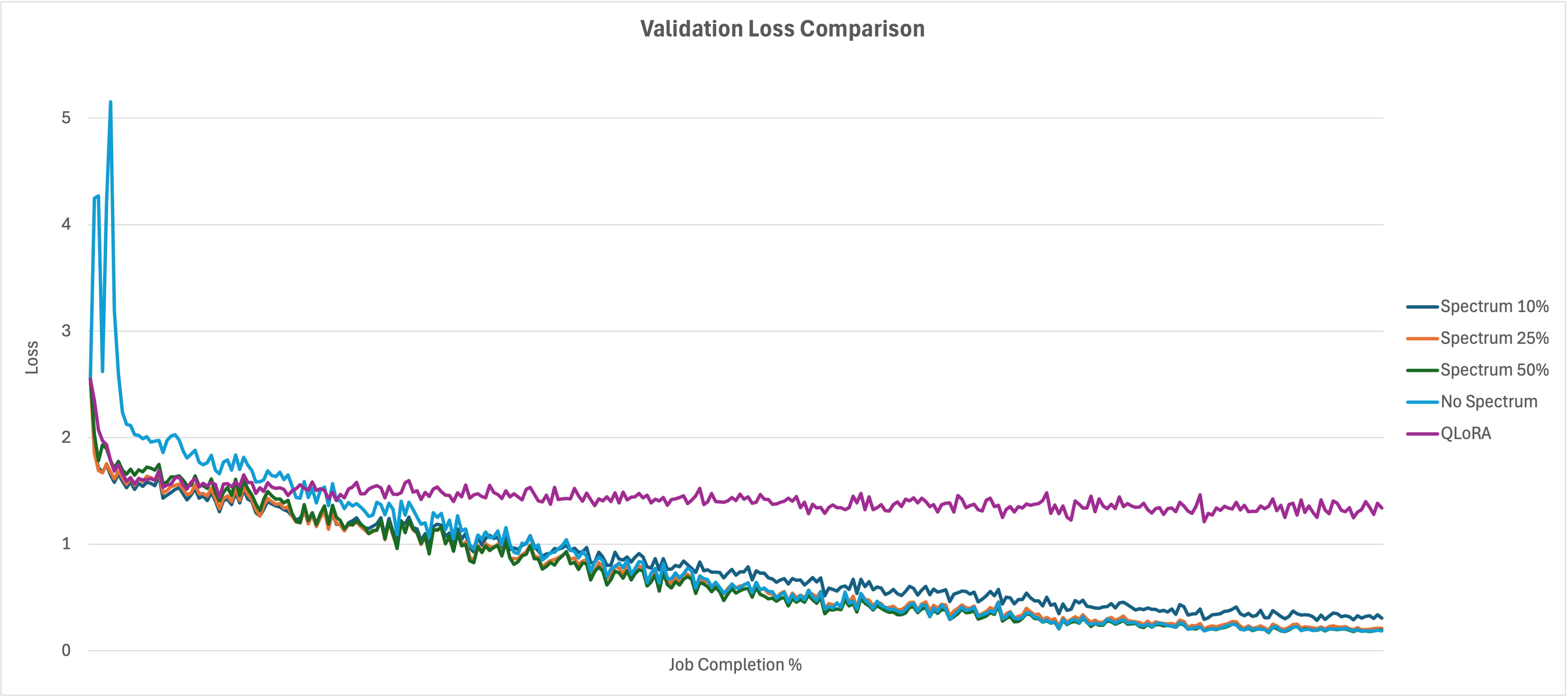
Summarizing the results from the following chart, you can see that QLoRA is the most efficient methodology in resource utilization and training time, but comes at a penalty to model quality (validation loss). It uses less memory than Spectrum at 10% for GPU and CPU, but comes at 778% loss penalty. The Spectrum runs converged relatively close to the No Spectrum run (between 0.006 and 0.121 difference), using less resources and cutting training time by between 25 and 58 percent. This shows how effective training the most impactful layers can be, and while QLoRA is more resource efficient, it comes with an impact to accuracy.

Conclusion

In this post, you learned how you can reduce the resource requirements for fine-tuning a FM while reducing training time and retaining a high level of accuracy by using Spectrum to direct training updates to designated layers based on the Signal to Noise Ratio in full precision. You also learned how you can use the Amazon SageMaker Python SDK ModelTrainer class and Amazon SageMaker AI fully managed training jobs to quickly spin up training jobs on demand.

To learn more about the details of Spectrum, refer to the HuggingFace paper Spectrum: Targeted Training on Signal to Noise Ratio and to learn more about training on Amazon SageMaker AI, refer to the SageMaker AI documentation.

To get started using Spectrum, the SageMaker Distributed Training GitHub repository has the example code used in this post and has everything you need to train your own models.

About the authors

Mona Mona currently works as a Sr World Wide Gen AI Specialist Solutions Architect at Amazon focusing on Gen AI Solutions in Amazon SageMaker AI team. She is a published author of two books – Natural Language Processing with AWS AI Services and Google Cloud Certified Professional Machine Learning Study Guide. She has authored 20+ blogs on AI/ML and cloud technology and a co-author on a research paper on CORD19 Neural Search which won an award for Best Research Paper at the prestigious AAAI (Association for the Advancement of Artificial Intelligence) conference.

Giuseppe Zappia is a Principal AI/ML Specialist Solutions Architect at AWS, focused on helping large enterprises design and deploy ML solutions on AWS. He has over 20 years of experience as a full stack software engineer, and has spent the past 6 years at AWS focused on the field of machine learning.

Amin Dashti is a Senior Data Scientist and researcher at AWS who bridges deep theoretical insight with practical machine learning expertise. With a background in theoretical physics and over seven years of experience, he has designed and deployed scalable models across domains — from predictive analytics and statistical inference in financial systems to cutting-edge applications in computer vision (CV) and natural language processing (NLP).