Artificial Intelligence
Forecasting financial time series with dynamic deep learning on AWS
Forecasting the evolution of events over time is essential to many applications, such as option pricing, disease progression, speech recognition, and supply chain management. It is also notoriously difficult: The goal is not just to predict an overall outcome but instead a precise sequence of events that will happen at specific times. Niels Bohr, a physics Nobel laureate, famously said that “prediction is very difficult, especially if it’s about the future.” In this blog post I will explore advanced techniques for time series forecasting using deep learning approaches on AWS. The post focuses on arbitrary time series value prediction so will be of interest to any reader working with time series. The post assumes that the reader already possesses basic technical knowledge in the field of Machine Learning.
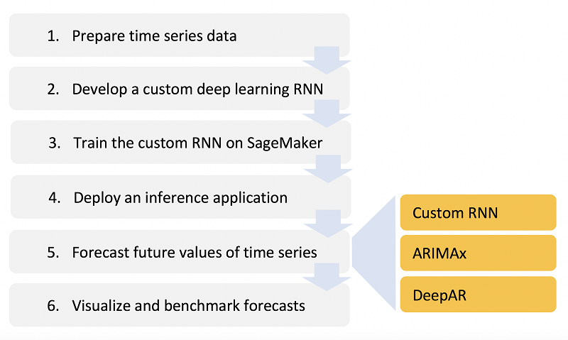
In this post, I will show you how to develop an original RNN (Recurrent Neural Network) deep learning algorithm to forecast time series based on the past trends of multiple factors, taking advantage of Amazon SageMaker (using Bring-Your-Own-Algorithm). Amazon SageMaker is a fully-managed machine learning platform that enables data scientists and developers to quickly and easily build and train machine learning models into production applications, at scale. It enables you to use both built-in algorithms, built-in frameworks, and also import custom code via Docker containers.
After developing a custom algorithm, I will show how to carry benchmark analyses to evaluate its performance. I will implement a version of ARIMA (Auto Regressive Integrated Moving Average) adapted for inclusion of co-factors. ARIMA is a standard, linear forecasting method (i.e. the equivalent of linear regression in the context of time series analysis, see details in the “Visualize and benchmark forecasts” section), often used as reference benchmark for time series forecasting. SageMaker released a first version of a built-in time series forecasting method based on RNN called DeepAR, so I’ll also compare performance of the custom model with DeepAR.
The goal of this blog is not to prove that one forecasting method is better than the other but to show you how to develop a custom model and benchmark it against standard methods until better generalization performance is achieved. There is indeed a tradeoff to choose between convenience and control: developing a custom deep learning algorithm allows full control over the details of its network architecture (e.g. a combination of multiple sub-networks) and parameterization (e.g. type of recurrent units, loss function, and activation functions). DeepAR in contrast is pre-built and as such the easiest and fastest way to forecast time series based on deep learning technology. Developing your own custom model will require more time, but it will provide you with endless options for fine tuning the performance.
The code needed to replicate all the results in this blog post is provided here. Upload the entire directory in a SageMaker instance, open the notebook named SageMakerNotebook.ipynb, and simply execute each cell one after the other. You shouldn’t have to change the code, just follow instructions inside this notebook.
The data is considered to be financial time series in $ and could, for example, represent revenues, profits, costs, stocks, interests and so forth. Goal will be to forecast the daily value of a series A over a sequence of 10 days, based on five factors: (1) the past trend of its own values, (2) the past trend of its own transaction volumes, (3) the past trend of another series values, (4) the past trend of the other series volumes, (5) and the past trend of the market sentiment as inferred from top news headlines every day. Of course, the code could be adapted to forecast the future trend of any time series, based on the past trends of any other related factors. For now though this blog will show you how to develop an original custom RNN model, implement ARIMA, use DeepAR, and evaluate their performance at predicting financial time series based on 5 factors, all in the same SageMaker notebook. Let’s get started!
Introduction to time series analysis and dynamic deep learning
Forecasting the dynamics of sequential events, i.e. time series, can be carried out using different methods depending on how much detail we know on the probability distribution of the data we aim to forecast. Fitting a probability distribution to the data enables to formulate past and future trends of a time series simply as the results of a parametric equation. If we had a perfectly known probability function for all quantities we aim to forecast, for a given initial value all solutions at all times could be found (Fig.2). For example, when trying to predict a stock value, if we knew all factors that influence this stock and could formulate a probability function that governs the relationship between all these factors, this function would tell us everything we want to know. Of course, we almost never have this function. So we use numeric approximation (Fig.2), by discretizing time into small intervals and computing the evolution of values (called states) one after the other based on available information. Information generally used to predict the future includes trends within the past evolution of states, randomness (i.e. variability around trends) and boundary conditions (e.g. origin of an epidemic, strike price of an option).
Figure 2: Discretization of a dynamic system into finite states and formulation of future trends as a function of trends observed in the past
Traditional approaches in the financial services sector rely either on the past trends of a given stock or on the finite difference or stochastic (random) sampling around a pre-defined probability formulation. In contrast, dynamic deep learning (i.e. recurrent neural Networks, RNN) enables inferences based on the trends of multiple correlated variables (e.g. stocks, market sentiment) without any assumption on their probability distribution. To do so, deep learning leverages the short and long-term memory of micro-/macro-cycles observed in the past by training the model to learn what matters and what doesn’t in these trends over large amounts of data. Key to RNN is the presence of a delay unit depicted on Fig.3, which memorizes the state at a given time step and re-injects it into the deep layers at the next time step, and so forth, recurrently over a chosen period of time (called lags). The algorithm learns to infer a sequence of future values (called horizon) based on a given lag by learning over multiple pairs of lag-horizon taken across the available timeline. This is referred to as sequence to sequence learning. The recurrence equation can make the network very deep because it replicates the entire hidden network at every step and leads to vanishing memory (i.e. the influence of the deepest layers vanishes due to repeated multiplications of small number derivatives needed to reach these layers during the process of gradient optimization). Some more advanced gated systems have been proposed to help with the vanishing memory issue, such as the GRU depicted in Fig.3. The idea behind GRU is to re-inject prior time-step learning into more recent time-step learning to benefit from both long term and short term memory.
Figure 3: Architecture of recurrent neural networks and gated recurrent units (GRU) that help solve vanishing memory issues as explained in the text
Prepare time series data
In this blog post we use the daily values of time series derived by randomizing time series available between 2010 and 2016 from the public repository Yahoo Finance. In the code shown below, we extract the entire time line for four related time series (SERIES A values and volumes, SERIES B values and volumes).
These are then differenced by order 1 to make the series approximately stationary (current series tend to increase over time), normalized and split in overlapping pairs of lag-horizons. The horizon was chosen to be 10 days, and since a rule of thumb in sequence-to-sequence learning is to choose a lag larger than the horizon, the lag was set to 3 weeks (note this could be further optimized through hyperparameter optimization (HPO)). 90% of the time line was used to sample pairs of lag-horizons for training. The remaining 10% was used later on (see section 5) to define non-overlapping pairs of lag-horizons and assess the performance of the model.
Overall market sentiment is known to affect business transaction (such as individual spending levels and mass trading) and can thus influence daily financial time series. So in addition to the four time series above, we also use a dataset publicly available on Kaggle that gathers some of the top daily news headlines between 2008 and 2016, extract a sentiment polarity that ranges somewhere between -1 (very unhappy) and 1 (very happy) for each headline and sum this index over all headlines, every day, to engineer a daily time series for overall market sentiment. Same format is applied as for the four time series earlier. This defines a fifth time series that we hypothesize is related to SERIES A and B and can thereby potentially help forecasting.
All five time series can be fed in the RNN as a 3D tensor where the third dimension is time.
In the rest of this post, we show how RNN can be used to train a model that infers the future time evolution of the SERIES A values based on its past trends (including volumes) as well as the past trend of another SERIES B, and market sentiment. Then we compare the results with those obtained from ARIMAx and DeepAR.
Develop a custom deep learning RNN
In the excerpt shown below, an RNN architecture is designed using the Keras API with TensorFlow backend that merges two sub-RNN, each with a layer of 256 gated recurrent units. The first sub-RNN aims entirely at forecasting future trends of the target series (SERIES A values) based on its own past, while the second sub-RNN aims at forecasting the same target series but based on the past of the four other time series (SERIES A volume, SERIES B values and volumes, and market sentiment). The two sub-RNN are combined together by branching into a final dense layer through a weight w assigned to one sub-RNN and its complementary (1-w) assigned to the other sub-RNN. This becomes a hyperparameter that provides control on how much to use the main time series versus co-factor time series when making predictions. Different w values were briefly tested. Values in the range 0.5 – 0.8 (which favors information coming from the sub-RNN trained on the target series) tend to produce best results (note this could be further optimized through HPO).
Train the RNN on SageMaker
After the data pipeline and RNN design have been implemented (file named Train), a SageMaker notebook can be used to import all necessary packages for the session, define the session, upload the data on Amazon S3, build a Docker container and push it on Amazon ECR, and finally train the RNN model. Note how SageMaker lets you create an estimator with the model and request specific Amazon EC2 resources in just one line.
Deploy an inference application
As when training the model, SageMaker provides an easy setup (you can do it in just one line) for creating an endpoint and deploying the model on an inference application. There is also flexibility on the type and the number of EC2 instances running in backend. For this blog post we will use a general purpose EC2 instance. The CSV serializer can also be used to pass diverse data format into CSV format to the model behind the endpoint.
Forecast future values of time series
To produce forecasts from the inference endpoint, the code is similar to the data pipeline implemented during training where the five time series (SERIES A values and volumes, SERIES B values and volumes, and market sentiment) are differenced to make them approximately stationary, normalized and split in overlapping pairs of lag-horizons (see details in section 1). There are two key differences: (i) The scaling/normalization step for a new time series (a new observation in 2D ML parlance) is not made in isolation but with reference to the scale of the original training data. The intuition here is that a trained model has defined its own coordinate system for each input feature so any new observation needs be translated in that same coordinate system. Since in our example the training data is not too large and readily available we just re-import this set when scaling a new observation. And (ii) after the forecast is produced we transform the results back to the original scale. The forecasting step itself simply consists of calling the pre-trained model with the data formatted as described earlier.
As when training the model, after the data has been prepared and put in the right format, SageMaker provides an easy setup for using the model online by invoking the endpoint created earlier. It forecasts SERIES A values based on the most recent trend (lags) of SERIES A volumes, SERIES B values and volumes, and market sentiment. This again with flexibility on the type and the number of EC2 instances running in the backend.
Visualize and benchmark forecasts
To evaluate the performance of a time series forecasting model we follow the same principles as in any other machine learning approach, that is we compare predicted against observed values. This provides us with a confidence level for any forecasts we might make in the future. To generalize well, this validation phase should be done on a sample of lag-horizon pairs that have never been seen when the model was trained to fit its parameters because ultimately the model aims to be used on previously unseen lags data. This sample also should contain many observations, although in sequence-to-sequence learning an observation is made of multiple predicted values because there are multiple time steps in an horizon, in contrast to non-dynamic ML approaches.
In our example, we kept 10% of the original time line for validation purposes, which corresponds to the period from May to December 2016, and uniformly sampled 4 pairs of non-overlapping lag-horizon pairs during this period to capture a diverse set of observed trends. For each sample Fig.4 compares the 10-day forecasted horizon with the actual, observed values. The mean absolute error (MAE) was used to penalize the magnitude of the error independently of its sign, and preferred to mean squared error (MSE) because we are more interested in trends over multiple points than in how large a particular point’s error might be. MAE for each sample is respectively $10, $24, $14, and $15. That’s $16 on average, which corresponds to MAE < 3% relative to SERIES A values. Note the news headlines data was not available after 7/1/2016 in the Kaggle dataset so only the first sample uses this feature, which the RNN combo elegantly accommodates without having to change its architectural design.
Figure 4: Performance of the custom RNN combo over four out-of-sample non-overlapping lag-horizon periods. MAE for each sample is respectively $10, $24, $14, and $15.
To thoroughly evaluate the performance of a time series forecasting model, it’s best to apply other methods and benchmark the results obtained with the different methods against each other. The code to implement ARIMAx and DeepAR and apply these two methods onto the same data as the custom RNN combo is provided in the attached files.
In the case of ARIMAx, which is ARIMA adapted for the inclusion of co-factors, a prediction at time t is made by regressing a target time series on (i) some lag p of the time series itself and other related time series, which is the deterministic part, AR, and (ii) some lag q of random fluctuations around the moving average along the time series itself and other related time series, which is the stochastic part, MA. In equation this gives:
where x is a set of time series, e the random fluctuation around the time series moving average and (a,b) the weighting parameters (same concept as weights in standard regression models). The time series can be differenced (i.e. integrated) by any order to make them stationary before to apply AR and MA, hence the name AR-I-MA. The x suffix stands for exogenous variables, which here are simply the other four related time series (SERIES A volumes, SERIES B values and volumes, sentiment) after we shift the dates in the past by a number of time steps corresponding to the horizon, see code in attached files. As shown in Fig.5, the SERIES A values do not seem auto-correlated with the previous 2 time steps, but both the SERIES A volumes and volatility (as modeled by the MA term in the earlier equation and accounted for in the partial auto-correlation function (PACF) curve) are auto-correlated beyond white noise up to 3 time steps.
Figure 5: Auto-correlation function (ACF, left) and partial auto-correlation function (PACF, right) of series A value and volume across the entire available time span
Looking at the ACF and PACF in Fig. 5 can help you choose proper values of the parameters p and q. I ran a grid search over all possible combinations of (p,q) within the [2,6] range for sample 1 and found that (p,d,q) = (4,0,4) produces the best results. See code/results in the attached files. The results from ARIMAx applied on same data as used for RNN combo with (p,d,q) = (4,0,4) are shown in Fig. 6 and Fig. 7.
In Fig. 6 we see a key benefit of ARIMA in forecasting time series, which is to provide a linear mapping between input and output with a set of weights (see column Estimate) that can be used to assess the importance of each input time series. In particular, we see the SERIES B values significantly impacts forecasts made for SERIES A values. The market sentiment (s) does too but to a lower extent, and volumes are relatively insignificant for the purpose of forecasting the SERIES A values with ARIMAx. In Fig.7 we see a key limitation of ARIMA: It is a linear forecasting approach and tends to not generalize well when trends are significantly non-linear. In our example, we see that the forecasts from ARIMAx remain quantitatively reasonable after 10 days but completely miss daily and other micro-cyclic trends which could lead to high errors if these micro-cycles were more pronounced or if the target horizon was larger than 10 days.
Figure 6: Description of best performer ARIMAx model after training
Recently, Amazon SageMaker released a first version of a built-in time series forecasting method based on RNN called DeepAR, which in current release has some advantages that lie in-between ARIMAx and the RNN combo developed here. Of course the Amazon SageMaker DeepAR possesses a key advantage which is to be pre-built and thereby the fastest and easiest to use on SageMaker. With limited time, this is the recommended approach on SageMaker. But as explained in the introduction there is a tradeoff to choose between convenience and control. In the case of DeepAR, the user may set hyper-parameters such as the number of layers, number of recurrent units in each layer, and learning rate. The user does not control hyper-parameters such as the nature of the activation functions in the different neurons, type of optimizers/loss functions, type of recurrent units (e.g. GRU vs. LSTM), and more generally the network architecture itself. So the user does not control how different time series are fed in the network, and in fact in the current release the product team recommends to not use co-factors if their values can’t be known over the horizon period. Sometimes the value of co-factors can indeed be known in advance, such as how many press releases Amazon will post in the next 10 days. But oftentimes, such as in our use case, we want to leverage co-factors such as different product revenues or different stocks and market sentiment for which value is known in the past but not in the future.
In this circumstance, the goal of this article is not to prove that one forecasting method is better than the other but to show how to develop a custom deep learning RNN model and benchmark it against standard methods such as ARIMAx and DeepAR until better performance is achieved with available time series. Since the DeepAR product team does not recommend the use of co-factors in the past, I trained the DeepAR with SERIES A and SERIES B values and market sentiment mostly for illustrative purpose. Note that a new version of DeepAR will soon be released that allows more flexibility when working with co-factors.
Figures 7: Benchmark analysis: Visualization of forecasts produced by the RNN combo, ARIMAx and DeepAR together with what was actually observed for the series A values
The results of Fig.7 do not prove that one method performs better than the other as explained earlier, but they do suggest that the custom RNN combo might perform better than DeepAR, likely because less features are used in DeepAR as explained earlier, and it surely performs better than ARIMAx. It’s evident from Fig.7 that the RNN combo follows daily trends more closely than ARIMAx (the forecast from ARIMAx is close to a straight line).
Conclusion
This blog post shows you how to develop a deep learning RNN architecture and customize it for a specific use case, implement two additional forecasting methods, ARIMAx and DeepAR, and benchmark performance results using the Amazon SageMaker elastically scalable and production ready environment. The use case chosen here was forecasting the future time evolution of a financial time series based on the past trends of this series as well as the past trends of multiple other factors, namely other time series values and overall market sentiment. The code in attached file can be adapted to other use cases and other time series with minimal changes.
About the Author
 Jeremy David Curuksu is a data scientist and consultant at the Amazon’s Machine Learning Solutions Lab. He holds a MSc and a PhD in applied mathematics, and was a research scientist at EPFL (Switzerland) and MIT (US). He is the author of multiple scientific peer-reviewed articles and the book Data Driven, which introduces management consulting in the new age of data science.