Build a cold start time series forecasting engine using AutoGluon

November 2022: This post is now obsolete. Please refer to the latest blog post Easy and accurate forecasting with AutoGluon-TimeSeries.

Whether you’re allocating resources more efficiently for web traffic, forecasting patient demand for staffing needs, or anticipating sales of a company’s products, forecasting is an essential tool across many businesses. One particular use case, known as cold start forecasting, builds forecasts for a time series that has little or no existing historical data, such as a new product that just entered the market in the retail industry. Traditional time series forecasting methods such as autoregressive integrated moving average (ARIMA) or exponential smoothing (ES) rely heavily on historical time series of each individual product, and therefore aren’t effective for cold start forecasting.

In this post, we will demonstrate how to build a cold start forecasting engine using AutoGluon AutoML for time AutoGluon AutoML for time series forecasting (preview), an open-source Python package to automate machine learning on image, text, tabular, and time series data. AutoGluon provides an end-to-end AutoML pipeline for beginners to experienced ML developers, making it the most accurate and easy-to-use fully automated solution. We will leverage the free Amazon SageMaker Studio Lab service for this demonstration.

Introduction to AutoGluon time series

AutoGluon is a leading open-source library for AutoML for text, image, and tabular data, allowing you to produce highly accurate models from raw data with just one line of code. Recently, the team has been working to extend these capabilities to time series data, and has developed an automated forecasting module that is publicly available on GitHub. The autogluon.forecasting module automatically processes raw time series data into the appropriate format, and then trains and tunes various state-of-the-art deep learning models to produce accurate forecasts. In this post, we demonstrate how to use autogluon.forecasting and apply it to cold start forecasting tasks.

Solution overview

Because AutoGluon is an open-source Python package, you can implement this solution locally on your laptop or on Amazon SageMaker Studio Lab. We walk through the following steps:

1. Set up AutoGluon for Amazon SageMaker Studio Lab.
2. Prepare the dataset.
3. Define training parameters using AutoGluon.
4. Train a cold start forecasting engine for time series forecasting.
5. Visualize cold start forecasting predictions.

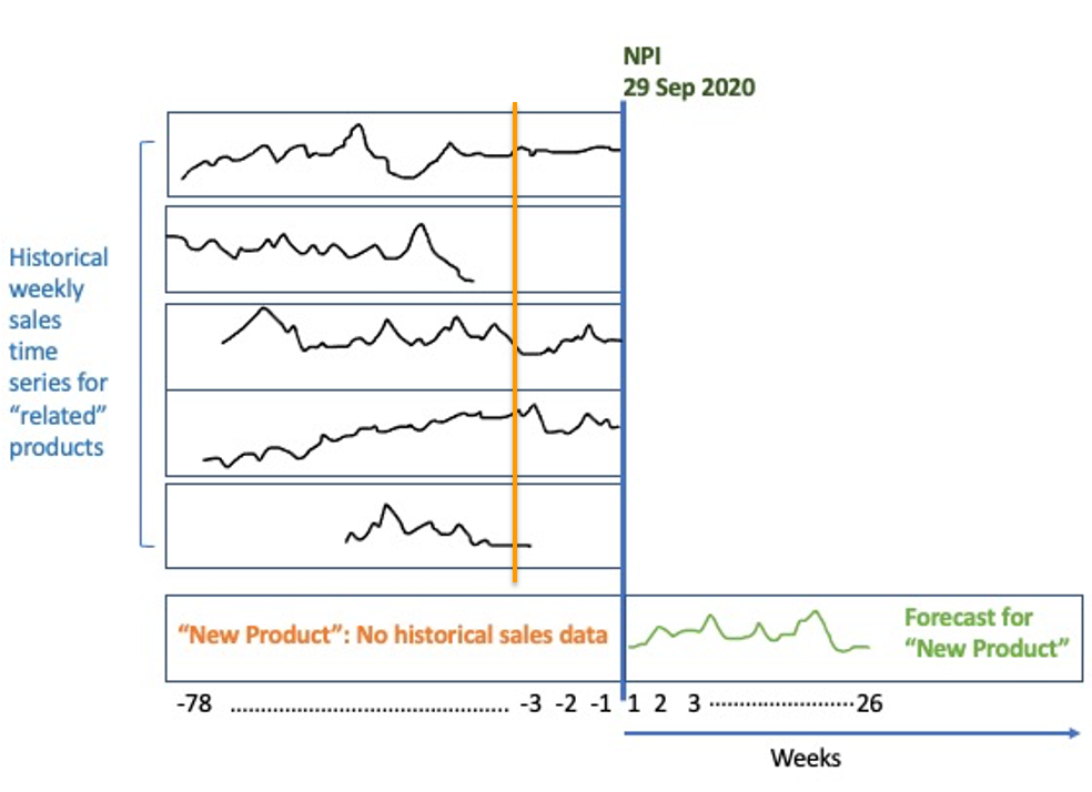
The key assumption of cold start forecasting is that items with similar characteristics should have similar time series trajectories, which is what allows cold start forecasting to make predictions on items without historical data, as illustrated in the following figure.

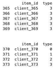
In our walkthrough, we use a synthetic dataset based on electricity consumption, which consists of the hourly time series for 370 items, each with an item_id from 0–369. Within this synthetic dataset, each item_id is also associated with a static feature (a feature that doesn’t change over time). We train a DeepAR model using AutoGluon to learn the typical behavior of similar items, and transfer such behavior to make predictions on new items (item_id 370–373) that don’t have historical time series data. Although we’re demonstrating the cold start forecasting approach with only one static feature, in practice, having informative and high-quality static features is the key for a good cold start forecast.

The following diagram provides a high-level overview of our solution. The open-source code is available on the GitHub repo.

Prerequisites

For this walkthrough, you should have the following prerequisites:

• An Amazon SageMaker Studio Lab account
• GitHub account access

Log in to your Amazon SageMaker Studio Lab account and set up the environment using the terminal:

cd sagemaker-studiolab-notebooks/ 
git clone https://github.com/whosivan/amazon-sagemaker-studio-lab-cold-start-forecasting-using-autogluon
conda env create -f autogluon.yml
conda activate autogluon
git clone https://github.com/yx1215/autogluon.git
cd autogluon/
git checkout --track origin/add_forecasting_predictor

These instructions should also work from your laptop if you don’t have access to Amazon SageMaker Studio Lab (we recommend installing Anaconda on your laptop first).

When you have the virtual environment fully set up, launch the notebook AutoGluon-cold-start-demo.ipynb and select the custom environment .conda-autogluon:Python kernel.

Prepare the target time series and item meta dataset

Download the following datasets to your notebook instance if they’re not included, and save them under the directory data/. You can find these datasets on our GitHub repo:

• Test.csv.gz
• coldStartTargetData.csv
• itemMetaData.csv

Run the following snippet to load the target time series dataset into the kernel:

zipLocalFilePath = "data/test.csv.gz"
localFilePath = "data/test.csv"
util.extract_gz(zipLocalFilePath, localFilePath)

tdf = pd.read_csv(zipLocalFilePath, dtype = object)
tdf['target_value'] = tdf['target_value'].astype('float')
tdf.head()

AutoGluon time series requires static features to be represented in numerical format. This can be achieved through applying LabelEncoder() on our static feature type, where we encode A=0, B=1, C=2, D=3 (see the following code). By default, AutoGluon infers the static feature to be either ordinal or categorical. You can also overwrite this by converting the static feature column to be the object/string data type for categorical features, or integer/float data type for ordinal features.

localItemMetaDataFilePath = "data/itemMetaData.csv"
imdf = pd.read_csv(localItemMetaDataFilePath, dtype = object)

labelencoder = LabelEncoder()
imdf['type'] = labelencoder.fit_transform(imdf['type'])

imdf_without_coldstart_item['type'] = imdf_without_coldstart_item['type'].astype(str)

imdf_without_coldstart_item = imdf[imdf.item_id.isin(tdf.item_id.tolist())]
imdf_without_coldstart_item.to_csv('data/itemMetaDatawithoutColdstart.csv', index=False)

imdf_with_coldstart_item = imdf[~imdf.item_id.isin(tdf.item_id.tolist())]
imdf_with_coldstart_item.to_csv('data/itemMetaDataOnlyColdstart.csv', index=False)

Set up and start AutoGluon model training

We need to specify save_path = ‘autogluon-coldstart-demo’ as the model artifact folder name (see the following code). We also set our eval_metric as mean absolute percentage error, or ‘MAPE’ for short, where we defined prediction_length as 24 hours. If not specified, AutoGluon by default produces probabilistic forecasts and scores them via the weighted quantile loss. We only look at the DeepAR model in our demo, because we know the DeepAR algorithm allows cold start forecasting by design. We set one of the DeepAR hyperparameters arbitrarily and pass that hyperparameter to the ForecastingPredictor().fit() call. This allows AutoGluon to look only into the specified model. For a full list of tunable hyperparameters, refer to gluonts.model.deepar package.

save_path = 'autogluon-coldstart-demo'
eval_metric = 'MAPE'
deepar_params = {
    "scaling":True
}

ag_predictor = ForecastingPredictor(path=save_path, 
eval_metric=eval_metric).fit(tdf, static_features = imdf_without_coldstart_item,
prediction_length=24, #how far out in the future we wish to forecast                                                                  index_column="item_id",                             
target_column="target_value",                                          
time_column="timestamp",
quantiles=[0.1, 0.5, 0.9],                                                                
hyperparameters={"DeepAR": deepar_params})

The training takes 30–45 minutes. You can get the model summary by calling the following function:

ag_predictor.fit_summary()

Forecast on the cold start item

Now we’re ready to generate forecasts for the cold start item. We recommend having at least five rows for each item_id. Therefore, for the item_id that has fewer than five observations, we fill in with NaNs. In our demo, both item_id 370 and 372 have zero observation, a pure cold start problem, whereas the other two have five target values.

Load in the cold start target time series dataset with the following code:

localColdStartDataFilePath = "data/coldStartTargetData.csv"
cstdf = pd.read_csv(localColdStartDataFilePath, dtype = object)
cstdf.head(20)

We feed the cold start target time series into our AutoGluon model, along with the item meta dataset for the cold start item_id:

cold_start_prediction = ag_predictor.predict(cstdf, static_features=imdf_with_coldstart_item)

Visualize the predictions

We can create a plotting function to generate a visualization on the cold start forecasting, as shown in the following graph.

Clean up

To optimize resource usage, consider stopping the runtime on Amazon SageMaker Studio Lab after you have fully explored the notebook.

Conclusion

In this post, we showed how to build a cold start forecasting engine using AutoGluon AutoML for time series data on Amazon SageMaker Studio Lab. For those of you who are wondering the difference between Amazon Forecast and AutoGluon (time series), Amazon Forecast is a fully managed and supported service that uses machine learning (ML) to generate highly accurate forecasts without requiring any prior ML experience. While AutoGluon is an open-source project that is community supported with the latest research contributions. We walked through an end-to-end example to demonstrate what AutoGluon for time series is capable of, and provided a dataset and use case.

AutoGluon for time series data is an open-source Python package, and we hope that this post, together with our code example, gives you a straightforward solution to tackle challenging cold start forecasting problems. You can access the entire example on our GitHub repo. Try it out, and let us know what you think!

About the Authors

Ivan Cui is a Data Scientist with AWS Professional Services, where he helps customers build and deploy solutions using machine learning on AWS. He has worked with customers across diverse industries, including software, finance, pharmaceutical, and healthcare. In his free time, he enjoys reading, spending time with his family, and maximizing his stock portfolio.

Jonas Mueller is a Senior Applied Scientist in the AI Research and Education group at AWS, where he develops new algorithms to improve deep learning and develop automated machine learning. Before joining AWS to democratize ML, he completed his PhD at the MIT Computer Science and Artificial Intelligence Lab. In his free time, he enjoys exploring mountains and the outdoors.

Wenming Ye is a Research Product Manager at AWS AI. He is passionate about helping researchers and enterprise customers rapidly scale their innovations through open-source and state-of-the-art machine learning technology. Wenming has diverse R&D experience from Microsoft Research, the SQL engineering team, and successful startups.