Collecting and annotating image data is one of the most resource-intensive tasks on any computer vision project. It can take months at a time to fully collect, analyze, and experiment with image streams at the level you need in order to compete in the current marketplace. Even after you’ve successfully collected data, you still have a constant stream of annotation errors, poorly framed images, small amounts of meaningful data in a sea of unwanted captures, and more. These major bottlenecks are why synthetic data creation needs to be in the toolkit of every modern engineer. By creating 3D representations of the objects we want to model, we can rapidly prototype algorithms while concurrently collecting live data.
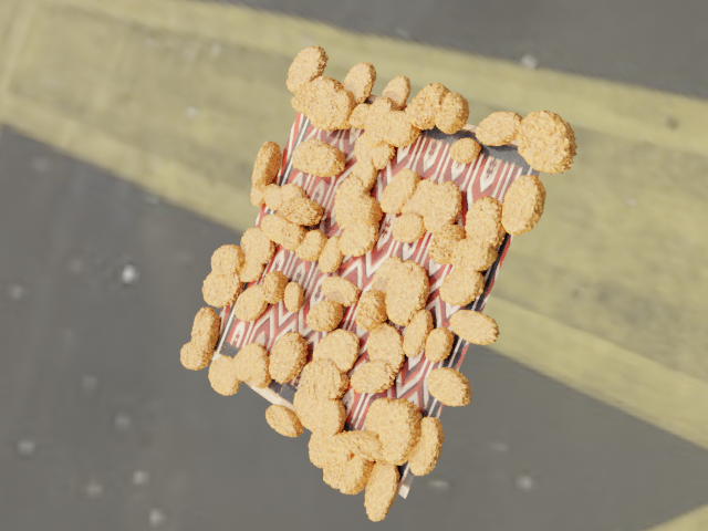
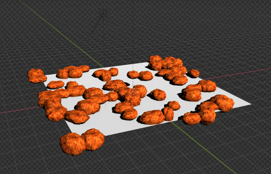
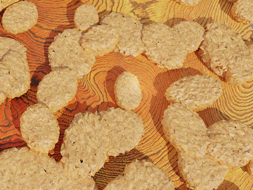
In this post, I walk you through an example of using the open-source animation library Blender to build an end-to-end synthetic data pipeline, using chicken nuggets as an example. The following image is an illustration of the data generated in this blog post.
What is Blender?
Blender is an open-source 3D graphics software primarily used in animation, 3D printing, and virtual reality. It has an extremely comprehensive rigging, animation, and simulation suite that allows the creation of 3D worlds for nearly any computer vision use case. It also has an extremely active support community where most, if not all, user errors are solved.
Set up your local environment
We install two versions of Blender: one on a local machine with access to a GUI, and the other on an Amazon Elastic Compute Cloud (Amazon EC2) P2 instance.
Install Blender and ZPY
Install Blender from the Blender website.
Then complete the following steps:
- Run the following commands:
wget https://mirrors.ocf.berkeley.edu/blender/release/Blender3.2/blender-3.2.0-linux-x64.tar.xz
sudo tar -Jxf blender-3.2.0-linux-x64.tar.xz --strip-components=1 -C /bin
rm -rf blender*

/bin/3.2/python/bin/python3.10 -m ensurepip
/bin/3.2/python/bin/python3.10 -m pip install --upgrade pip
- Copy the necessary Python headers into the Blender version of Python so that you can use other non-Blender libraries:
wget https://www.python.org/ftp/python/3.10.2/Python-3.10.2.tgz
tar -xzf Python-3.10.2.tgz
sudo cp Python-3.10.2/Include/* /bin/3.2/python/include/python3.10
- Override your Blender version and force installs so that the Blender-provided Python works:
/bin/3.2/python/bin/python3.10 -m pip install pybind11 pythran Cython numpy==1.22.1
sudo /bin/3.2/python/bin/python3.10 -m pip install -U Pillow --force
sudo /bin/3.2/python/bin/python3.10 -m pip install -U scipy --force
sudo /bin/3.2/python/bin/python3.10 -m pip install -U shapely --force
sudo /bin/3.2/python/bin/python3.10 -m pip install -U scikit-image --force
sudo /bin/3.2/python/bin/python3.10 -m pip install -U gin-config --force
sudo /bin/3.2/python/bin/python3.10 -m pip install -U versioneer --force
sudo /bin/3.2/python/bin/python3.10 -m pip install -U shapely --force
sudo /bin/3.2/python/bin/python3.10 -m pip install -U ptvsd --force
sudo /bin/3.2/python/bin/python3.10 -m pip install -U ptvseabornsd --force
sudo /bin/3.2/python/bin/python3.10 -m pip install -U zmq --force
sudo /bin/3.2/python/bin/python3.10 -m pip install -U pyyaml --force
sudo /bin/3.2/python/bin/python3.10 -m pip install -U requests --force
sudo /bin/3.2/python/bin/python3.10 -m pip install -U click --force
sudo /bin/3.2/python/bin/python3.10 -m pip install -U table-logger --force
sudo /bin/3.2/python/bin/python3.10 -m pip install -U tqdm --force
sudo /bin/3.2/python/bin/python3.10 -m pip install -U pydash --force
sudo /bin/3.2/python/bin/python3.10 -m pip install -U matplotlib --force
- Download
zpy and install from source:
git clone https://github.com/ZumoLabs/zpy
cd zpy
vi requirements.txt
- Change the NumPy version to
>=1.19.4 and scikit-image>=0.18.1 to make the install on 3.10.2 possible and so you don’t get any overwrites:
numpy>=1.19.4
gin-config>=0.3.0
versioneer
scikit-image>=0.18.1
shapely>=1.7.1
ptvsd>=4.3.2
seaborn>=0.11.0
zmq
pyyaml
requests
click
table-logger>=0.3.6
tqdm
pydash
- To ensure compatibility with Blender 3.2, go into
zpy/render.py and comment out the following two lines (for more information, refer to Blender 3.0 Failure #54):
#scene.render.tile_x = tile_size
#scene.render.tile_y = tile_size
- Next, install the
zpy library:
/bin/3.2/python/bin/python3.10 setup.py install --user
/bin/3.2/python/bin/python3.10 -c "import zpy; print(zpy.__version__)"
- Download the add-ons version of
zpy from the GitHub repo so you can actively run your instance:
cd ~
curl -O -L -C - "https://github.com/ZumoLabs/zpy/releases/download/v1.4.1rc9/zpy_addon-v1.4.1rc9.zip"
sudo unzip zpy_addon-v1.4.1rc9.zip -d /bin/3.2/scripts/addons/
mkdir .config/blender/
mkdir .config/blender/3.2
mkdir .config/blender/3.2/scripts
mkdir .config/blender/3.2/scripts/addons/
mkdir .config/blender/3.2/scripts/addons/zpy_addon/
sudo cp -r zpy/zpy_addon/* .config/blender/3.2/scripts/addons/zpy_addon/
- Save a file called
enable_zpy_addon.py in your /home directory and run the enablement command, because you don’t have a GUI to activate it:
import bpy, os
p = os.path.abspath('zpy_addon-v1.4.1rc9.zip')
bpy.ops.preferences.addon_install(overwrite=True, filepath=p)
bpy.ops.preferences.addon_enable(module='zpy_addon')
bpy.ops.wm.save_userpref()

sudo blender -b -y --python enable_zpy_addon.py
If zpy-addon doesn’t install (for whatever reason), you can install it via the GUI.
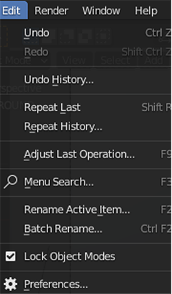
- In Blender, on the Edit menu, choose Preferences.
- Choose Add-ons in the navigation pane and activate
zpy.
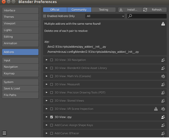
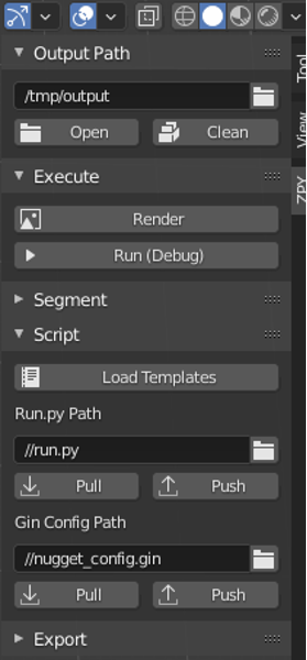
You should see a page open in the GUI, and you’ll be able to choose ZPY. This will confirm that Blender is loaded.
AliceVision and Meshroom
Install AliceVision and Meshrooom from their respective GitHub repos:
FFmpeg
Your system should have ffmpeg, but if it doesn’t, you’ll need to download it.
Instant Meshes
You can either compile the library yourself or download the available pre-compiled binaries (which is what I did) for Instant Meshes.
Set up your AWS environment
Now we set up the AWS environment on an EC2 instance. We repeat the steps from the previous section, but only for Blender and zpy.
- On the Amazon EC2 console, choose Launch instances.
- Choose your AMI.There are a few options from here. We can either choose a standard Ubuntu image, pick a GPU instance, and then manually install the drivers and get everything set up, or we can take the easy route and start with a preconfigured Deep Learning AMI and only worry about installing Blender.For this post, I use the second option, and choose the latest version of the Deep Learning AMI for Ubuntu (Deep Learning AMI (Ubuntu 18.04) Version 61.0).
- For Instance type¸ choose p2.xlarge.
- If you don’t have a key pair, create a new one or choose an existing one.
- For this post, use the default settings for network and storage.
- Choose Launch instances.
- Choose Connect and find the instructions to log in to our instance from SSH on the SSH client tab.
- Connect with SSH:
ssh -i "your-pem" ubuntu@IPADDRESS.YOUR-REGION.compute.amazonaws.com
Once you’ve connected to your instance, follow the same installation steps from the previous section to install Blender and zpy.
Data collection: 3D scanning our nugget
For this step, I use an iPhone to record a 360-degree video at a fairly slow pace around my nugget. I stuck a chicken nugget onto a toothpick and taped the toothpick to my countertop, and simply rotated my camera around the nugget to get as many angles as I could. The faster you film, the less likely you get good images to work with depending on the shutter speed.
After I finished filming, I sent the video to my email and extracted the video to a local drive. From there, I used ffmepg to chop the video into frames to make Meshroom ingestion much easier:
mkdir nugget_images
ffmpeg -i VIDEO.mov ffmpeg nugget_images/nugget_%06d.jpg
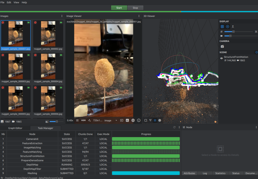
Open Meshroom and use the GUI to drag the nugget_images folder to the pane on the left. From there, choose Start and wait a few hours (or less) depending on the length of the video and if you have a CUDA-enabled machine.
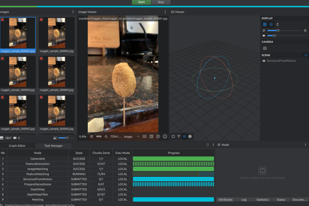
You should see something like the following screenshot when it’s almost complete.
Data collection: Blender manipulation
When our Meshroom reconstruction is complete, complete the following steps:
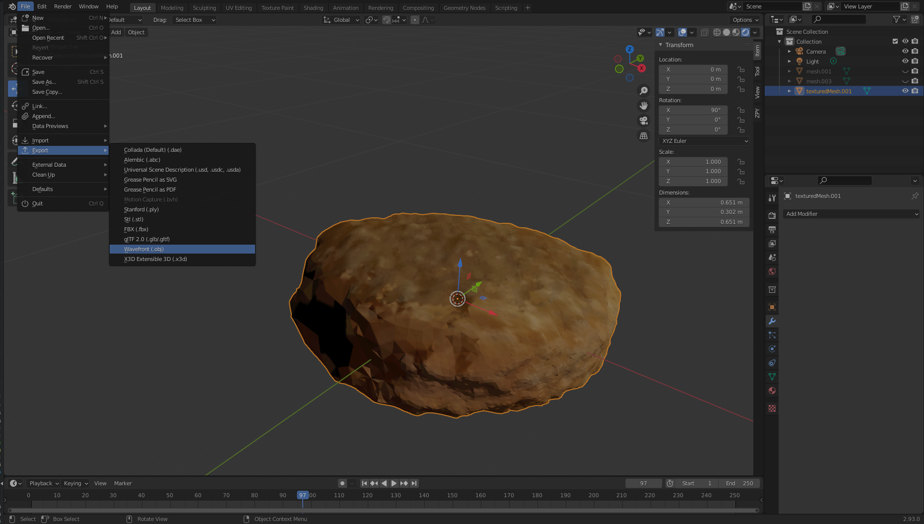
- Open the Blender GUI and on the File menu, choose Import, then choose Wavefront (.obj) to your created texture file from Meshroom.
The file should be saved in path/to/MeshroomCache/Texturing/uuid-string/texturedMesh.obj.
- Load the file and observe the monstrosity that is your 3D object.
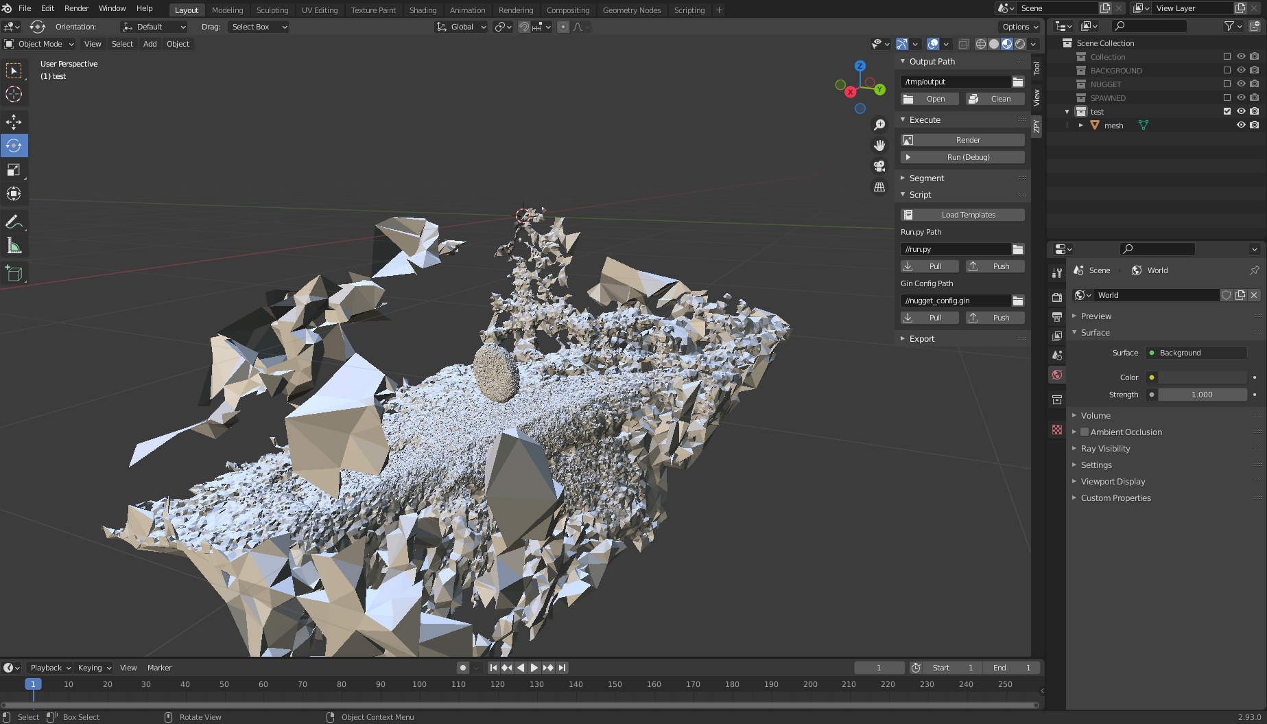
Here is where it gets a bit tricky.
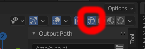
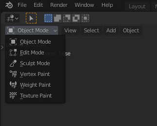
- Scroll to the top right side and choose the Wireframe icon in Viewport Shading.
- Select your object on the right viewport and make sure it’s highlighted, scroll over to the main layout viewport, and either press Tab or manually choose Edit Mode.
- Next, maneuver the viewport in such a way as to allow yourself to be able to see your object with as little as possible behind it. You’ll have to do this a few times to really get it correct.
- Click and drag a bounding box over the object so that only the nugget is highlighted.
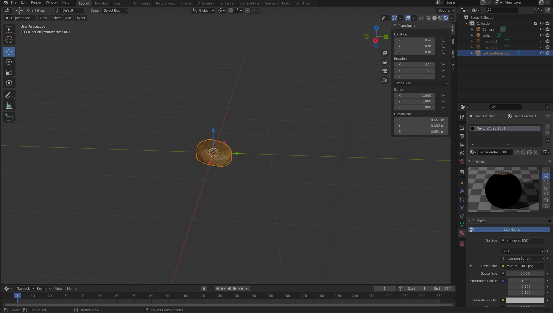
- After it’s highlighted like in the following screenshot, we separate our nugget from the 3D mass by left-clicking, choosing Separate, and then Selection.
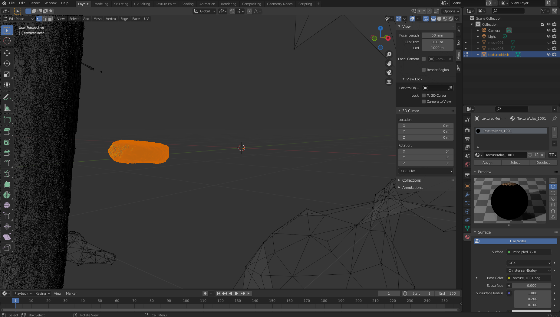
We now move over to the right, where we should see two textured objects: texturedMesh and texturedMesh.001.
- Our new object should be
texturedMesh.001, so we choose texturedMesh and choose Delete to remove the unwanted mass.
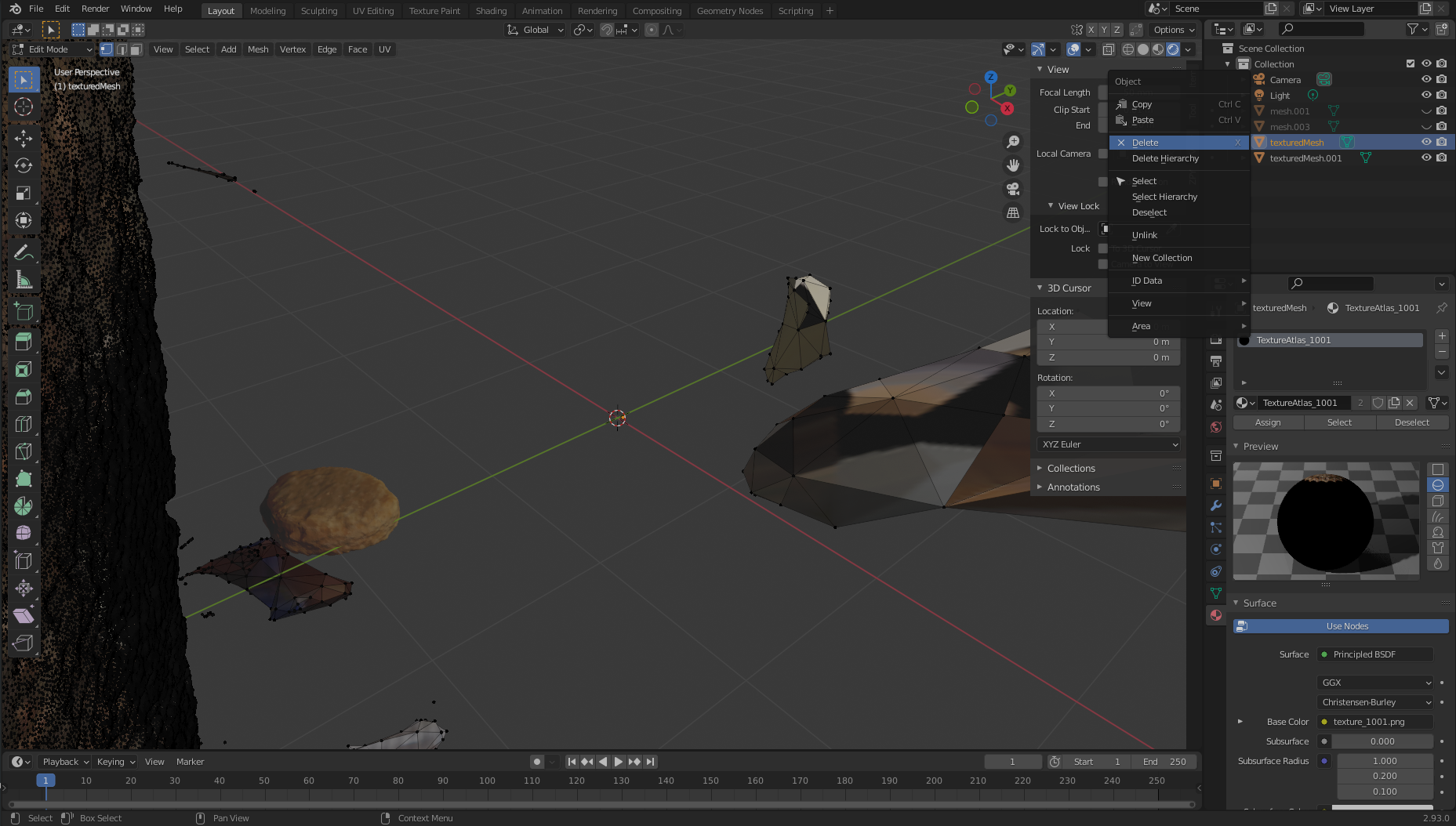
- Choose the object (
texturedMesh.001) on the right, move to our viewer, and choose the object, Set Origin, and Origin to Center of Mass.
Now, if we want, we can move our object to the center of the viewport (or simply leave it where it is) and view it in all its glory. Notice the large black hole where we didn’t really get good film coverage from! We’re going to need to correct for this.
To clean our object of any pixel impurities, we export our object to an .obj file. Make sure to choose Selection Only when exporting.
Data collection: Clean up with Instant Meshes
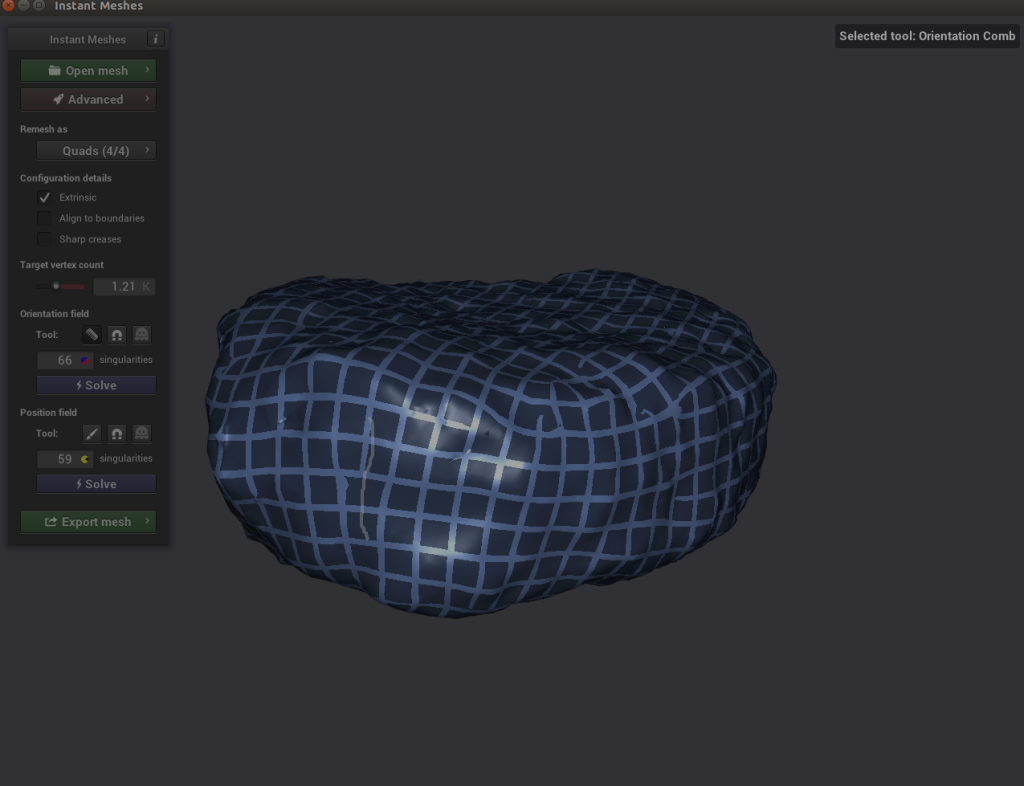
Now we have two problems: our image has a pixel gap creating by our poor filming that we need to clean up, and our image is incredibly dense (which will make generating images extremely time-consuming). To tackle both issues, we need to use a software called Instant Meshes to extrapolate our pixel surface to cover the black hole and also to shrink the total object to a smaller, less dense size.
- Open Instant Meshes and load our recently saved
nugget.obj file.
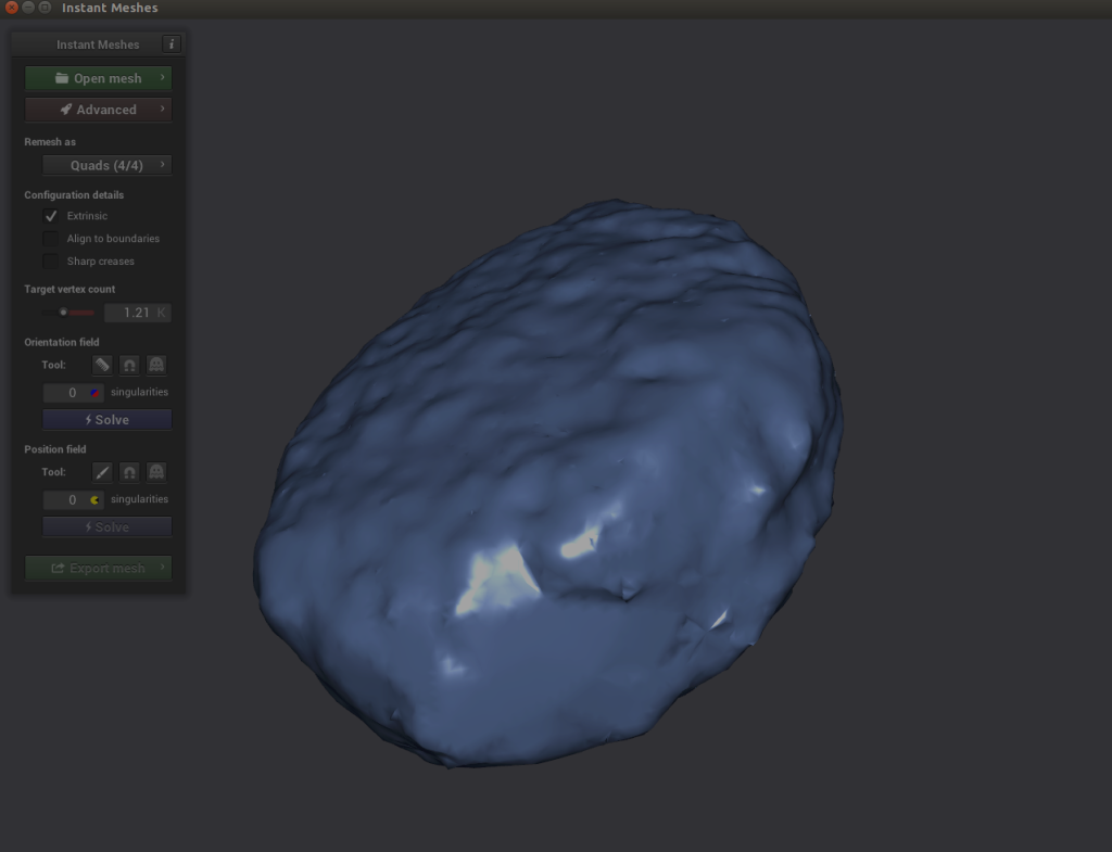
- Under Orientation field, choose Solve.
- Under Position field, choose Solve.
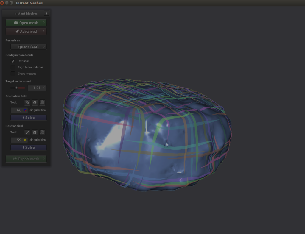
 Here’s where it gets interesting. If you explore your object and notice that the criss-cross lines of the Position solver look disjointed, you can choose the comb icon under Orientation field and redraw the lines properly.
- Choose Solve for both Orientation field and Position field.
- If everything looks good, export the mesh, name it something like
nugget_refined.obj, and save it to disk.
Data collection: Shake and bake!
Because our low-poly mesh doesn’t have any image texture associated with it and our high-poly mesh does, we either need to bake the high-poly texture onto the low-poly mesh, or create a new texture and assign it to our object. For sake of simplicity, we’re going to create an image texture from scratch and apply that to our nugget.
I used Google image search for nuggets and other fried things in order to get a high-res image of the surface of a fried object. I found a super high-res image of a fried cheese curd and made a new image full of the fried texture.
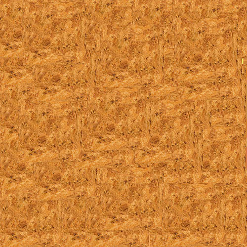
With this image, I’m ready to complete the following steps:
- Open Blender and load the new
nugget_refined.obj the same way you loaded your initial object: on the File menu, choose Import, Wavefront (.obj), and choose the nugget_refined.obj file.
- Next, go to the Shading tab.
At the bottom you should notice two boxes with the titles Principled BDSF and Material Output.
- On the Add menu, choose Texture and Image Texture.
An Image Texture box should appear.
- Choose Open Image and load your fried texture image.
- Drag your mouse between Color in the Image Texture box and Base Color in the Principled BDSF box.
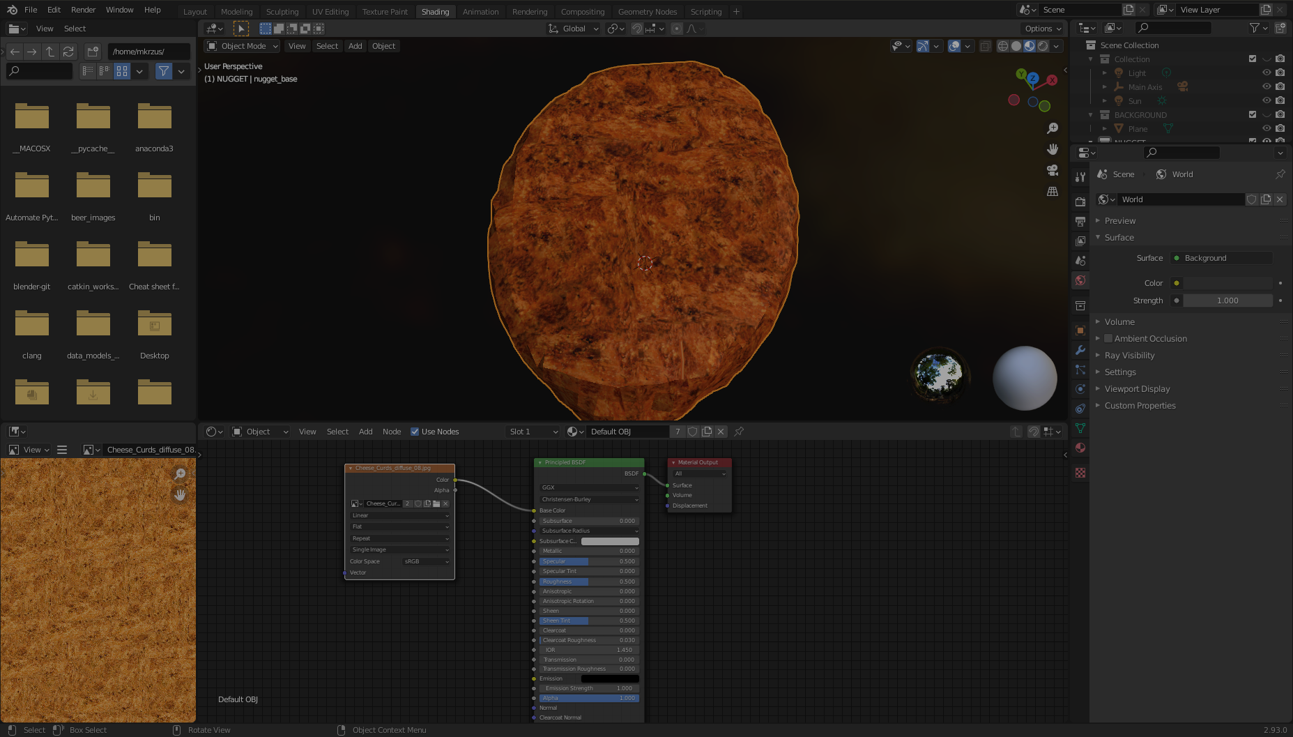
Now your nugget should be good to go!
Data collection: Create Blender environment variables
Now that we have our base nugget object, we need to create a few collections and environment variables to help us in our process.
- Left-click on the hand scene area and choose New Collection.
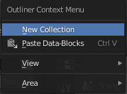
- Create the following collections: BACKGROUND, NUGGET, and SPAWNED.
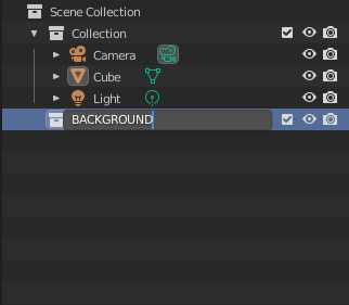
- Drag the nugget to the NUGGET collection and rename it nugget_base.
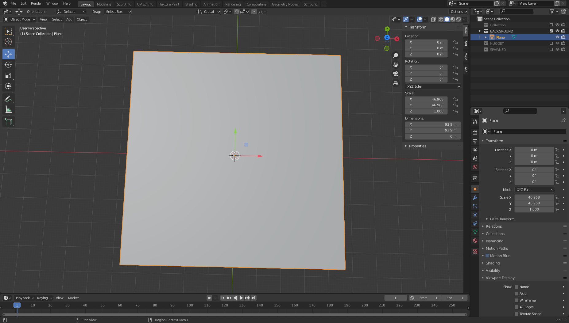
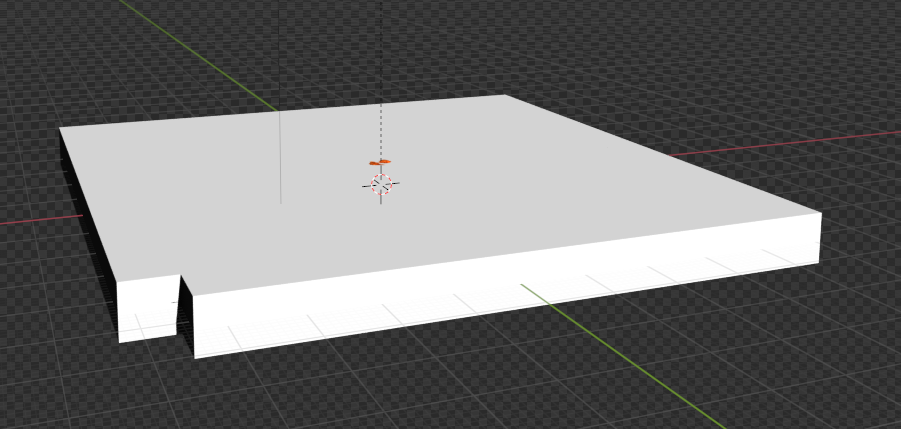
Data collection: Create a plane
We’re going to create a background object from which our nuggets will be generated when we’re rendering images. In a real-world use case, this plane is where our nuggets are placed, such as a tray or bin.
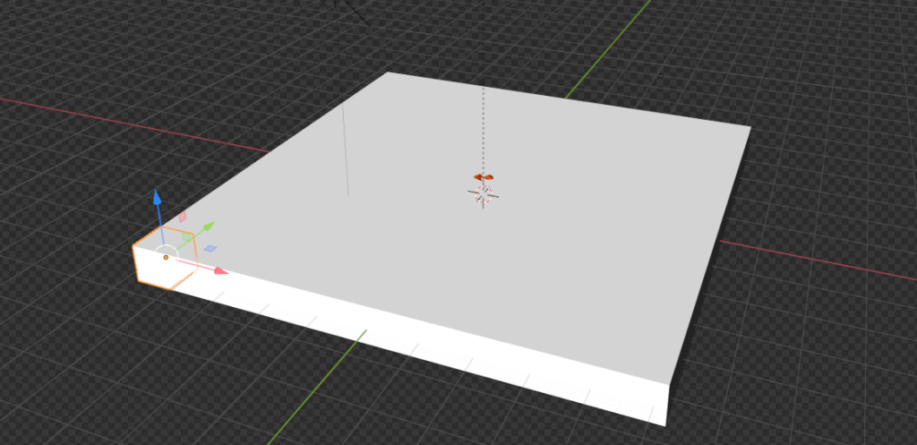
- On the Add menu, choose Mesh and then Plane.
From here, we move to the right side of the page and find the orange box (Object Properties).
- In the Transform pane, for XYZ Euler, set X to 46.968, Y to 46.968, and Z to 1.0.
- For both Location and Rotation, set X, Y, and Z to 0.
Data collection: Set the camera and axis
Next, we’re going to set our cameras up correctly so that we can generate images.
- On the Add menu, choose Empty and Plain Axis.
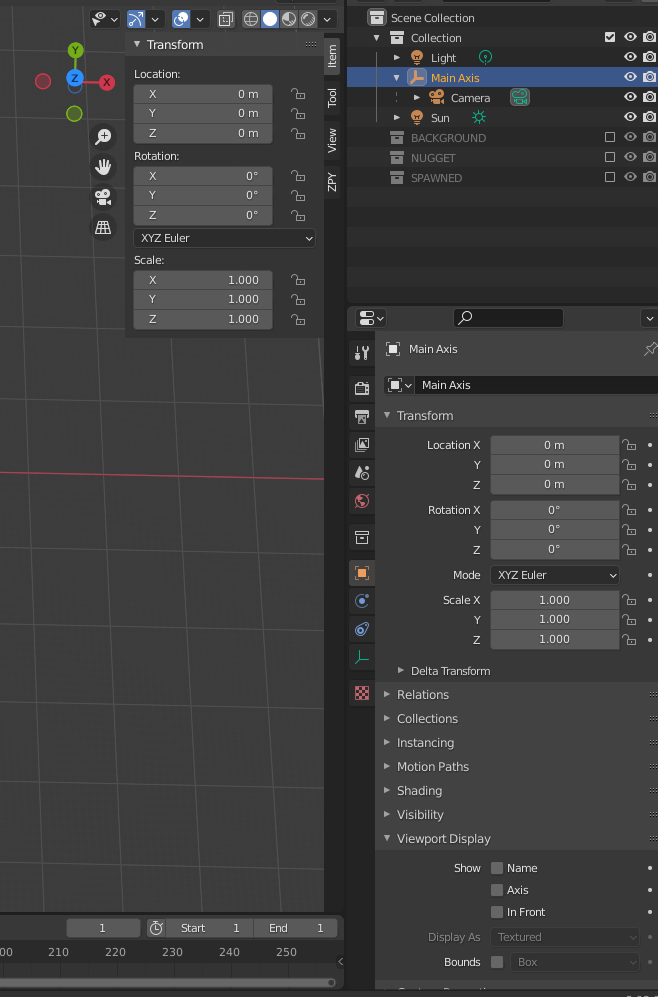
- Name the object Main Axis.
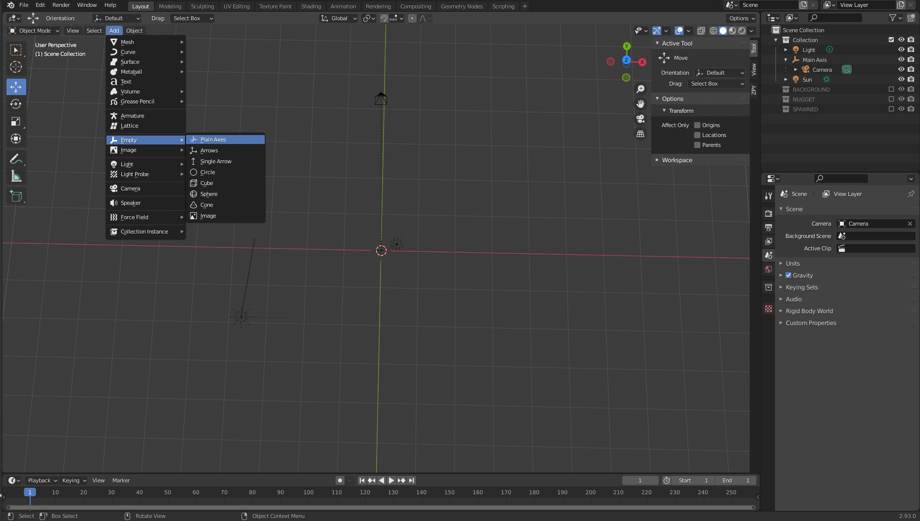
- Make sure our axis is 0 for all the variables (so it’s directly in the center).
- If you have a camera already created, drag that camera to under Main Axis.
- Choose Item and Transform.
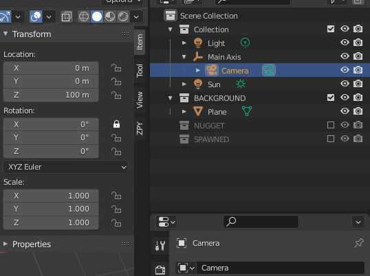
- For Location, set X to 0, Y to 0, and Z to 100.
Data collection: Here comes the sun
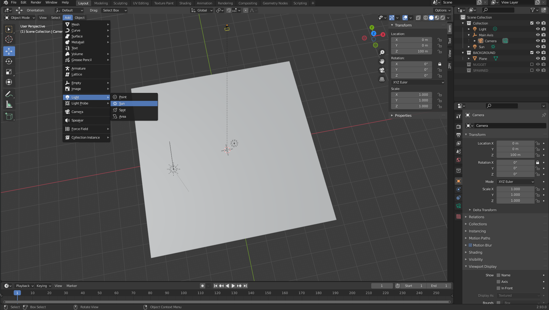
Next, we add a Sun object.
- On the Add menu, choose Light and Sun.
The location of this object doesn’t necessarily matter as long as it’s centered somewhere over the plane object we’ve set.
- Choose the green lightbulb icon in the bottom right pane (Object Data Properties) and set the strength to 5.0.
- Repeat the same procedure to add a Light object and put it in a random spot over the plane.
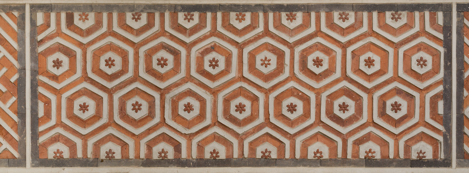
Data collection: Download random backgrounds
To inject randomness into our images, we download as many random textures from texture.ninja as we can (for example, bricks). Download to a folder within your workspace called random_textures. I downloaded about 50.
Generate images
Now we get to the fun stuff: generating images.
Image generation pipeline: Object3D and DensityController
Let’s start with some code definitions:
class Object3D:
	'''
	object container to store mesh information about the
	given object

	Returns
	the Object3D object
	'''
	def __init__(self, object: Union[bpy.types.Object, str]):
		"""Creates a Object3D object.

		Args:
		obj (Union[bpy.types.Object, str]): Scene object (or it's name)
		"""
		self.object = object
		self.obj_poly = None
		self.mat = None
		self.vert = None
		self.poly = None
		self.bvht = None
		self.calc_mat()
		self.calc_world_vert()
		self.calc_poly()
		self.calc_bvht()

	def calc_mat(self) -> None:
		"""store an instance of the object's matrix_world"""
		self.mat = self.object.matrix_world

	def calc_world_vert(self) -> None:
		"""calculate the verticies from object's matrix_world perspective"""
		self.vert = [self.mat @ v.co for v in self.object.data.vertices]
		self.obj_poly = np.array(self.vert)

	def calc_poly(self) -> None:
		"""store an instance of the object's polygons"""
		self.poly = [p.vertices for p in self.object.data.polygons]

	def calc_bvht(self) -> None:
		"""create a BVHTree from the object's polygon"""
		self.bvht = BVHTree.FromPolygons( self.vert, self.poly )

	def regenerate(self) -> None:
		"""reinstantiate the object's variables;
		used when the object is manipulated after it's creation"""
		self.calc_mat()
		self.calc_world_vert()
		self.calc_poly()
		self.calc_bvht()

	def __repr__(self):
		return "Object3D: " + self.object.__repr__()
We first define a basic container Class with some important properties. This class mainly exists to allow us to create a BVH tree (a way to represent our nugget object in 3D space), where we’ll need to use the BVHTree.overlap method to see if two independent generated nugget objects are overlapping in our 3D space. More on this later.
The second piece of code is our density controller. This serves as a way to bound ourselves to the rules of reality and not the 3D world. For example, in the 3D Blender world, objects in Blender can exist inside each other; however, unless someone is performing some strange science on our chicken nuggets, we want to make sure no two nuggets are overlapping by a degree that makes it visually unrealistic.
We use our Plane object to spawn a set of bounded invisible cubes that can be queried at any given time to see if the space is occupied or not.
See the following code:
class DensityController:
    """Container that controlls the spacial relationship between 3D objects

    Returns:
        DensityController: The DensityController object.
    """
    def __init__(self):
        self.bvhtrees = None
        self.overlaps = None
        self.occupied = None
        self.unoccupied = None
        self.objects3d = []

    def auto_generate_kdtree_cubes(
        self,
        num_objects: int = 100, # max size of nuggets
    ) -> None:
        """
        function to generate physical kdtree cubes given a plane of -resize- size
        this allows us to access each cube's overlap/occupancy status at any given
        time

        creates a KDTree collection, a cube, a set of individual cubes, and the
        BVHTree object for each individual cube

        Args:
            resize (Tuple[float]): the size of a cube to create XYZ.
            cuts (int): how many cuts are made to the cube face
                12 cuts == 13 Rows x 13 Columns
        """
In the following snippet, we select the nugget and create a bounding cube around that nugget. This cube represents the size of a single pseudo-voxel of our psuedo-kdtree object. We need to use the bpy.context.view_layer.update() function because when this code is being run from inside a function or script vs. the blender-gui, it seems that the view_layer isn’t automatically updated.
        # read the nugget,
        # see how large the cube needs to be to encompass a single nugget
        # then touch a parameter to allow it to be smaller or larger (eg more touching)
        bpy.context.view_layer.objects.active = bpy.context.scene.objects.get('nugget_base')
        bpy.ops.object.origin_set(type='ORIGIN_GEOMETRY', center='BOUNDS')
        #create a cube for the bounding box
        bpy.ops.mesh.primitive_cube_add(location=Vector((0,0,0)))
        #our new cube is now the active object, so we can keep track of it in a variable:
        bound_box = bpy.context.active_object
        bound_box.name = 'CUBE1'
        bpy.context.view_layer.update()
        #copy transforms
        nug_dims = bpy.data.objects["nugget_base"].dimensions
        bpy.data.objects["CUBE1"].dimensions = nug_dims
        bpy.context.view_layer.update()
        bpy.data.objects["CUBE1"].location = bpy.data.objects["nugget_base"].location
        bpy.context.view_layer.update()
        bpy.data.objects["CUBE1"].rotation_euler = bpy.data.objects["nugget_base"].rotation_euler
        bpy.context.view_layer.update()
        print("bound_box.dimensions: ", bound_box.dimensions)
        print("bound_box.location:", bound_box.location)
Next, we slightly update our cube object so that its length and width are square, as opposed to the natural size of the nugget it was created from:
        # this cube created isn't always square, but we're going to make it square
        # to fit into our
        x, y, z = bound_box.dimensions
        v = max(x, y)
        if np.round(v) < v:
            v = np.round(v)+1
        bb_x, bb_y = v, v
        bound_box.dimensions = Vector((v, v, z))
        bpy.context.view_layer.update()
        print("bound_box.dimensions updated: ", bound_box.dimensions)
        # now we generate a plane
        # calc the size of the plane given a max number of boxes.
Now we use our updated cube object to create a plane that can volumetrically hold num_objects amount of nuggets:
        x, y, z = bound_box.dimensions
        bb_loc = bound_box.location
        bb_rot_eu = bound_box.rotation_euler
        min_area = (x*y)*num_objects
        min_length = min_area / num_objects
        print(min_length)
        # now we generate a plane
        # calc the size of the plane given a max number of boxes.
        bpy.ops.mesh.primitive_plane_add(location=Vector((0,0,0)), size = min_length)
        plane = bpy.context.selected_objects[0]
        plane.name = 'PLANE'
        # move our plane to our background collection
        # current_collection = plane.users_collection
        link_object('PLANE', 'BACKGROUND')
        bpy.context.view_layer.update()
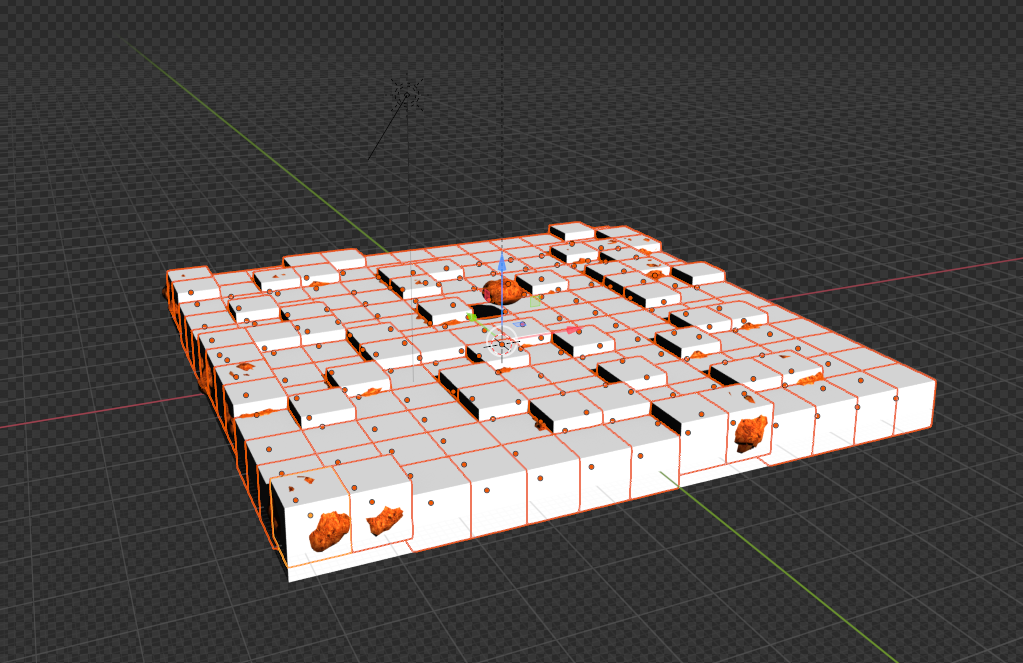
We take our plane object and create a giant cube of the same length and width as our plane, with the height of our nugget cube, CUBE1:
        # New Collection
        my_coll = bpy.data.collections.new("KDTREE")
        # Add collection to scene collection
        bpy.context.scene.collection.children.link(my_coll)
        # now we generate cubes based on the size of the plane.
        bpy.ops.mesh.primitive_cube_add(location=Vector((0,0,0)), size = min_length)
        bpy.context.view_layer.update()
        cube = bpy.context.selected_objects[0]
        cube_dimensions = cube.dimensions
        bpy.context.view_layer.update()
        cube.dimensions = Vector((cube_dimensions[0], cube_dimensions[1], z))
        bpy.context.view_layer.update()
        cube.location = bb_loc
        bpy.context.view_layer.update()
        cube.rotation_euler = bb_rot_eu
        bpy.context.view_layer.update()
        cube.name = 'cube'
        bpy.context.view_layer.update()
        current_collection = cube.users_collection
        link_object('cube', 'KDTREE')
        bpy.context.view_layer.update()
From here, we want to create voxels from our cube. We take the number of cubes we would to fit num_objects and then cut them from our cube object. We look for the upward-facing mesh-face of our cube, and then pick that face to make our cuts. See the following code:
        # get the bb volume and make the proper cuts to the object
        bb_vol = x*y*z
        cube_vol = cube_dimensions[0]*cube_dimensions[1]*cube_dimensions[2]
        n_cubes = cube_vol / bb_vol
        cuts = n_cubes / ((x+y) / 2)
        cuts = int(np.round(cuts)) - 1 #
        # select the cube
        for object in bpy.data.objects:
            object.select_set(False)
        bpy.context.view_layer.update()
        for object in bpy.data.objects:
            object.select_set(False)
        bpy.data.objects['cube'].select_set(True) # Blender 2.8x
        bpy.context.view_layer.objects.active = bpy.context.scene.objects.get('cube')
        # set to edit mode
        bpy.ops.object.mode_set(mode='EDIT', toggle=False)
        print('edit mode success')
        # get face_data
        context = bpy.context
        obj = context.edit_object
        me = obj.data
        mat = obj.matrix_world
        bm = bmesh.from_edit_mesh(me)
        up_face = None
        # select upwards facing cube-face
        # https://blender.stackexchange.com/questions/43067/get-a-face-selected-pointing-upwards
        for face in bm.faces:
            if (face.normal-UP_VECTOR).length < EPSILON:
                up_face = face
                break
        assert(up_face)
        # subdivide the edges to get the perfect kdtree cubes
        bmesh.ops.subdivide_edges(bm,
                edges=up_face.edges,
                use_grid_fill=True,
                cuts=cuts)
        bpy.context.view_layer.update()
        # get the center point of each face
Lastly, we calculate the center of the top-face of each cut we’ve made from our big cube and create actual cubes from those cuts. Each of these newly created cubes represents a single piece of space to spawn or move nuggets around our plane. See the following code:
        face_data = {}
        sizes = []
        for f, face in enumerate(bm.faces):
            face_data[f] = {}
            face_data[f]['calc_center_bounds'] = face.calc_center_bounds()
            loc = mat @ face_data[f]['calc_center_bounds']
            face_data[f]['loc'] = loc
            sizes.append(loc[-1])
        # get the most common cube-z; we use this to determine the correct loc
        counter = Counter()
        counter.update(sizes)
        most_common = counter.most_common()[0][0]
        cube_loc = mat @ cube.location
        # get out of edit mode
        bpy.ops.object.mode_set(mode='OBJECT', toggle=False)
        # go to new colection
        bvhtrees = {}
        for f in face_data:
            loc = face_data[f]['loc']
            loc = mat @ face_data[f]['calc_center_bounds']
            print(loc)
            if loc[-1] == most_common:
                # set it back down to the floor because the face is elevated to the
                # top surface of the cube
                loc[-1] = cube_loc[-1]
                bpy.ops.mesh.primitive_cube_add(location=loc, size = x)
                cube = bpy.context.selected_objects[0]
                cube.dimensions = Vector((x, y, z))
                # bpy.context.view_layer.update()
                cube.name = "cube_{}".format(f)
                #my_coll.objects.link(cube)
                link_object("cube_{}".format(f), 'KDTREE')
                #bpy.context.view_layer.update()
                bvhtrees[f] = {
                    'occupied' : 0,
                    'object' : Object3D(cube)
                }
        for object in bpy.data.objects:
            object.select_set(False)
        bpy.data.objects['CUBE1'].select_set(True) # Blender 2.8x
        bpy.ops.object.delete()
        return bvhtrees
Next, we develop an algorithm that understands which cubes are occupied at any given time, finds which objects overlap with each other, and moves overlapping objects separately into unoccupied space. We won’t be able get rid of all overlaps entirely, but we can make it look real enough.
See the following code:
    def find_occupied_space(
        self,
        objects3d: List[Object3D],
    ) -> None:
        """
        discover which cube's bvhtree is occupied in our kdtree space

        Args:
            list of Object3D objects

        """
        count = 0
        occupied = []
        for i in self.bvhtrees:
            bvhtree = self.bvhtrees[i]['object']
            for object3d in objects3d:
                if object3d.bvht.overlap(bvhtree.bvht):
                    self.bvhtrees[i]['occupied'] = 1

    def find_overlapping_objects(
        self,
        objects3d: List[Object3D],
    ) -> List[Tuple[int]]:
        """
        returns which Object3D objects are overlapping

        Args:
            list of Object3D objects

        Returns:
            List of indicies from objects3d that are overlap
        """
        count = 0
        overlaps = []
        for i, x_object3d in enumerate(objects3d):
            for ii, y_object3d in enumerate(objects3d[i+1:]):
                if x_object3d.bvht.overlap(y_object3d.bvht):
                    overlaps.append((i, ii))
        return overlaps

    def calc_most_overlapped(
        self,
        overlaps: List[Tuple[int]]
    ) -> List[Tuple[int]]:
        """
        Algorithm to count the number of edges each index has
        and return a sorted list from most->least with the number
        of edges each index has.

        Args:
            list of indicies that are overlapping

        Returns:
            list of indicies with the total number of overlapps they have
            [index, count]
        """
        keys = {}
        for x,y in overlaps:
            if x not in keys:
                keys[x] = 0
            if y not in keys:
                keys[y] = 0
            keys[x]+=1
            keys[y]+=1
        # sort by most edges first
        index_counts = sorted(keys.items(), key=lambda x: x[1])[::-1]
        return index_counts

    def get_random_unoccupied(
        self
    ) -> Union[int,None]:
        """
        returns a randomly chosen unoccuped kdtree cube

        Return
            either the kdtree cube's key or None (meaning all spaces are
            currently occupied)
            Union[int,None]
        """
        unoccupied = []
        for i in self.bvhtrees:
            if not self.bvhtrees[i]['occupied']:
                unoccupied.append(i)
        if unoccupied:
            random.shuffle(unoccupied)
            return unoccupied[0]
        else:
            return None

    def regenerate(
        self,
        iterable: Union[None, List[Object3D]] = None
    ) -> None:
        """
        this function recalculates each objects world-view information
        we default to None, which means we're recalculating the self.bvhtree cubes

        Args:
            iterable (None or List of Object3D objects). if None, we default to
            recalculating the kdtree
        """
        if isinstance(iterable, list):
            for object in iterable:
                object.regenerate()
        else:
            for idx in self.bvhtrees:
                self.bvhtrees[idx]['object'].regenerate()
                self.update_tree(idx, occupied=0)

    def process_trees_and_objects(
        self,
        objects3d: List[Object3D],
    ) -> List[Tuple[int]]:
        """
        This function finds all overlapping objects within objects3d,
        calculates the objects with the most overlaps, searches within
        the kdtree cube space to see which cubes are occupied. It then returns
        the edge-counts from the most overlapping objects

        Args:
            list of Object3D objects
        Returns
            this returns the output of most_overlapped
        """
        overlaps = self.find_overlapping_objects(objects3d)
        most_overlapped = self.calc_most_overlapped(overlaps)
        self.find_occupied_space(objects3d)
        return most_overlapped

    def move_objects(
        self,
        objects3d: List[Object3D],
        most_overlapped: List[Tuple[int]],
        z_increase_offset: float = 2.,
    ) -> None:
        """
        This function iterates through most-overlapped, and uses
        the index to extract the matching object from object3d - it then
        finds a random unoccupied kdtree cube and moves the given overlapping
        object to that space. It does this for each index from the most-overlapped
        function

        Args:
            objects3d: list of Object3D objects
            most_overlapped: a list of tuples (index, count) - where index relates to
                where it's found in objects3d and count - how many times it overlaps
                with other objects
            z_increase_offset: this value increases the Z value of the object in order to
                make it appear as though it's off the floor. If you don't augment this value
                the object looks like it's 'inside' the ground plane
        """
        for idx, cnt in most_overlapped:
            object3d = objects3d[idx]
            unoccupied_idx = self.get_random_unoccupied()
            if unoccupied_idx:
                object3d.object.location =  self.bvhtrees[unoccupied_idx]['object'].object.location
                # ensure the nuggest is above the groundplane
                object3d.object.location[-1] = z_increase_offset
                self.update_tree(unoccupied_idx, occupied=1)

    def dynamic_movement(
        self,
        objects3d: List[Object3D],
        tries: int = 100,
        z_offset: float = 2.,
    ) -> None:
        """
        This function resets all objects to get their current positioning
        and randomly moves objects around in an attempt to avoid any object
        overlaps (we don't want two objects to be spawned in the same position)

        Args:
            objects3d: list of Object3D objects
            tries: int the number of times we want to move objects to random spaces
                to ensure no overlaps are present.
            z_offset: this value increases the Z value of the object in order to
                make it appear as though it's off the floor. If you don't augment this value
                the object looks like it's 'inside' the ground plane (see `move_objects`)
        """

        # reset all objects
        self.regenerate(objects3d)
        # regenerate bvhtrees
        self.regenerate(None)

        most_overlapped = self.process_trees_and_objects(objects3d)
        attempts = 0
        while most_overlapped:
            if attempts>=tries:
                break
            self.move_objects(objects3d, most_overlapped, z_offset)
            attempts+=1
            # recalc objects
            self.regenerate(objects3d)
            # regenerate bvhtrees
            self.regenerate(None)
            # recalculate overlaps
            most_overlapped = self.process_trees_and_objects(objects3d)

    def generate_spawn_point(
        self,
    ) -> Vector:
        """
        this function generates a random spawn point by finding which
        of the kdtree-cubes are unoccupied, and returns one of those

        Returns
            the Vector location of the kdtree-cube that's unoccupied
        """
        idx = self.get_random_unoccupied()
        print(idx)
        self.update_tree(idx, occupied=1)
        return self.bvhtrees[idx]['object'].object.location

    def update_tree(
        self,
        idx: int,
        occupied: int,
    ) -> None:
        """
        this function updates the given state (occupied vs. unoccupied) of the
        kdtree given the idx

        Args:
            idx: int
            occupied: int
        """
        self.bvhtrees[idx]['occupied'] = occupied
Image generation pipeline: Cool runnings
In this section, we break down what our run function is doing.
We initialize our DensityController and create something called a saver using the ImageSaver from zpy. This allows us to seemlessly save our rendered images to any location of our choosing. We then add our nugget category (and if we had more categories, we would add them here). See the following code:
@gin.configurable("run")
@zpy.blender.save_and_revert
def run(
    max_num_nuggets: int = 100,
    jitter_mesh: bool = True,
    jitter_nugget_scale: bool = True,
    jitter_material: bool = True,
    jitter_nugget_material: bool = False,
    number_of_random_materials: int = 50,
    nugget_texture_path: str = os.getcwd()+"/nugget_textures",
    annotations_path = os.getcwd()+'/nugget_data',
):
    """
    Main run function.
    """
    density_controller = DensityController()
    # Random seed results in unique behavior
    zpy.blender.set_seed(random.randint(0,1000000000))

    # Create the saver object
    saver = zpy.saver_image.ImageSaver(
        description="Image of the randomized Amazon nuggets",
        output_dir=annotations_path,
    )
    saver.add_category(name="nugget")
Next, we need to make a source object from which we spawn copy nuggets from; in this case, it’s the nugget_base that we created:
    # Make a list of source nugget objects
    source_nugget_objects = []
    for obj in zpy.objects.for_obj_in_collections(
        [
            bpy.data.collections["NUGGET"],
        ]
    ):
        assert(obj!=None)

        # pass on everything not named nugget
        if 'nugget_base' not in obj.name:
            print('passing on {}'.format(obj.name))
            continue
        zpy.objects.segment(obj, name="nugget", as_category=True) #color=nugget_seg_color
        print("zpy.objects.segment: check {}".format(obj.name))
        source_nugget_objects.append(obj.name)
Now that we have our base nugget, we’re going to save the world poses (locations) of all the other objects so that after each rendering run, we can use these saved poses to reinitialize a render. We also move our base nugget completely out of the way so that the kdtree doesn’t sense a space being occupied. Finally, we initialize our kdtree-cube objects. See the following code:
    # move nugget point up 10 z's so it won't collide with base-cube
    bpy.data.objects["nugget_base"].location[-1] = 10

    # Save the position of the camera and light
    # create light and camera
    zpy.objects.save_pose("Camera")
    zpy.objects.save_pose("Sun")
    zpy.objects.save_pose("Plane")
    zpy.objects.save_pose("Main Axis")
    axis = bpy.data.objects['Main Axis']
    print('saving poses')
    # add some parameters to this

    # get the plane-3d object
    plane3d = Object3D(bpy.data.objects['Plane'])

    # generate kdtree cubes
    density_controller.generate_kdtree_cubes()
The following code collects our downloaded backgrounds from texture.ninja, where they’ll be used to be randomly projected onto our plane:
    # Pre-create a bunch of random textures
    #random_materials = [
    #    zpy.material.random_texture_mat() for _ in range(number_of_random_materials)
    #]
    p = os.path.abspath(os.getcwd()+'/random_textures')
    print(p)
    random_materials = []
    for x in os.listdir(p):
        texture_path = Path(os.path.join(p,x))
        y = zpy.material.make_mat_from_texture(texture_path, name=texture_path.stem)
        random_materials.append(y)
    #print(random_materials[0])

    # Pre-create a bunch of random textures
    random_nugget_materials = [
        random_nugget_texture_mat(Path(nugget_texture_path)) for _ in range(number_of_random_materials)
    ]
Here is where the magic begins. We first regenerate out kdtree-cubes for this run so that we can start fresh:
    # Run the sim.
    for step_idx in zpy.blender.step():
        density_controller.generate_kdtree_cubes()

        objects3d = []
        num_nuggets = random.randint(40, max_num_nuggets)
        log.info(f"Spawning {num_nuggets} nuggets.")
        spawned_nugget_objects = []
        for _ in range(num_nuggets):
We use our density controller to generate a random spawn point for our nugget, create a copy of nugget_base, and move the copy to the randomly generated spawn point:
            # Choose location to spawn nuggets
            spawn_point = density_controller.generate_spawn_point()
            # manually spawn above the floor
            # spawn_point[-1] = 1.8 #2.0

            # Pick a random object to spawn
            _name = random.choice(source_nugget_objects)
            log.info(f"Spawning a copy of source nugget {_name} at {spawn_point}")
            obj = zpy.objects.copy(
                bpy.data.objects[_name],
                collection=bpy.data.collections["SPAWNED"],
                is_copy=True,
            )

            obj.location = spawn_point
            obj.matrix_world = mathutils.Matrix.Translation(spawn_point)
            spawned_nugget_objects.append(obj)
Next, we randomly jitter the size of the nugget, the mesh of the nugget, and the scale of the nugget so that no two nuggets look the same:
            # Segment the newly spawned nugget as an instance
            zpy.objects.segment(obj)

            # Jitter final pose of the nugget a little
            zpy.objects.jitter(
                obj,
                rotate_range=(
                    (0.0, 0.0),
                    (0.0, 0.0),
                    (-math.pi * 2, math.pi * 2),
                ),
            )

            if jitter_nugget_scale:
                # Jitter the scale of each nugget
                zpy.objects.jitter(
                    obj,
                    scale_range=(
                        (0.8, 2.0), #1.2
                        (0.8, 2.0), #1.2
                        (0.8, 2.0), #1.2
                    ),
                )

            if jitter_mesh:
                # Jitter (deform) the mesh of each nugget
                zpy.objects.jitter_mesh(
                    obj=obj,
                    scale=(
                        random.uniform(0.01, 0.03),
                        random.uniform(0.01, 0.03),
                        random.uniform(0.01, 0.03),
                    ),
                )

            if jitter_nugget_material:
                # Jitter the material (apperance) of each nugget
                for i in range(len(obj.material_slots)):
                    obj.material_slots[i].material = random.choice(random_nugget_materials)
                    zpy.material.jitter(obj.material_slots[i].material)
We turn our nugget copy into an Object3D object where we use the BVH tree functionality to see if our plane intersects or overlaps any face or vertices on our nugget copy. If we find an overlap with the plane, we simply move the nugget upwards on its Z axis. See the following code:
            # create 3d obj for movement
            nugget3d = Object3D(obj)

            # make sure the bottom most part of the nugget is NOT
            # inside the plane-object
            plane_overlap(plane3d, nugget3d)

            objects3d.append(nugget3d)
Now that all nuggets are created, we use our DensityController to move nuggets around so that we have a minimum number of overlaps, and those that do overlap aren’t hideous looking:
        # ensure objects aren't on top of each other
        density_controller.dynamic_movement(objects3d)
In the following code: we restore the Camera and Main Axis poses and randomly select how far the camera is to the Plane object:
        # Return camera to original position
        zpy.objects.restore_pose("Camera")
        zpy.objects.restore_pose("Main Axis")
        zpy.objects.restore_pose("Camera")
        zpy.objects.restore_pose("Main Axis")

        # assert these are the correct versions...
        assert(bpy.data.objects["Camera"].location == Vector((0,0,100)))
        assert(bpy.data.objects["Main Axis"].location == Vector((0,0,0)))
        assert(bpy.data.objects["Main Axis"].rotation_euler == Euler((0,0,0)))

        # alter the Z ditance with the camera
        bpy.data.objects["Camera"].location = (0, 0, random.uniform(0.75, 3.5)*100)
We decide how randomly we want the camera to travel along the Main Axis. Depending on if we want it to be mainly overhead or if we care very much about the angle from which it sees the board, we can adjust the top_down_mostly parameter depending on how well our training model is picking up the signal of “What even is a nugget anyway?”
        # alter the main-axis beta/gamma params
        top_down_mostly = False
        if top_down_mostly:
            zpy.objects.rotate(
                bpy.data.objects["Main Axis"],
                rotation=(
                    random.uniform(0.05, 0.05),
                    random.uniform(0.05, 0.05),
                    random.uniform(0.05, 0.05),
                ),
            )
        else:
            zpy.objects.rotate(
                bpy.data.objects["Main Axis"],
                rotation=(
                    random.uniform(-1., 1.),
                    random.uniform(-1., 1.),
                    random.uniform(-1., 1.),
                ),
            )

        print(bpy.data.objects["Main Axis"].rotation_euler)
        print(bpy.data.objects["Camera"].location)
In the following code, we do the same thing with the Sun object, and randomly pick a texture for the Plane object:
        # change the background material
        # Randomize texture of shelf, floors and walls
        for obj in bpy.data.collections["BACKGROUND"].all_objects:
            for i in range(len(obj.material_slots)):
                # TODO
                # Pick one of the random materials
                obj.material_slots[i].material = random.choice(random_materials)
                if jitter_material:
                    zpy.material.jitter(obj.material_slots[i].material)
                # Sets the material relative to the object
                obj.material_slots[i].link = "OBJECT"
        # Pick a random hdri (from the local textures folder for background background)
        zpy.hdris.random_hdri()
        # Return light to original position
        zpy.objects.restore_pose("Sun")

        # Jitter the light position
        zpy.objects.jitter(
            "Sun",
            translate_range=(
                (-5, 5),
                (-5, 5),
                (-5, 5),
            ),
        )
        bpy.data.objects["Sun"].data.energy = random.uniform(0.5, 7)
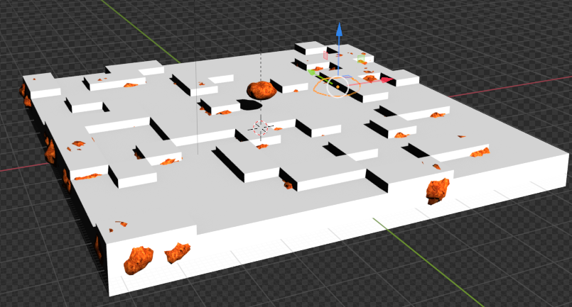
Finally, we hide all our objects that we don’t want to be rendered: the nugget_base and our entire cube structure:
# we hide the cube objects<br />for obj in         # we hide the cube objects
        for obj in bpy.data.objects:
            if 'cube' in obj.name:
                obj.hide_render = True
                try:
                    zpy.objects.toggle_hidden(obj, hidden=True)
                except:
                    # deal with this exception here...
                    pass
        # we hide our base nugget object
        bpy.data.objects["nugget_base"].hide_render = True
        zpy.objects.toggle_hidden(bpy.data.objects["nugget_base"], hidden=True)
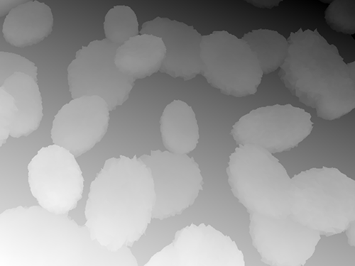
Lastly, we use zpy to render our scene, save our images, and then save our annotations. For this post, I made some small changes to the zpy annotation library for my specific use case (annotation per image instead of one file per project), but you shouldn’t have to for the purpose of this post).
        # create the image name
        image_uuid = str(uuid.uuid4())

        # Name for each of the output images
        rgb_image_name = format_image_string(image_uuid, 'rgb')
        iseg_image_name = format_image_string(image_uuid, 'iseg')
        depth_image_name = format_image_string(image_uuid, 'depth')

        zpy.render.render(
            rgb_path=saver.output_dir / rgb_image_name,
            iseg_path=saver.output_dir / iseg_image_name,
            depth_path=saver.output_dir / depth_image_name,
        )

        # Add images to saver
        saver.add_image(
            name=rgb_image_name,
            style="default",
            output_path=saver.output_dir / rgb_image_name,
            frame=step_idx,
        )

        saver.add_image(
            name=iseg_image_name,
            style="segmentation",
            output_path=saver.output_dir / iseg_image_name,
            frame=step_idx,
        )
        saver.add_image(
            name=depth_image_name,
            style="depth",
            output_path=saver.output_dir / depth_image_name,
            frame=step_idx,
        )

        # ideally in this thread, we'll open the anno file
        # and write to it directly, saving it after each generation
        for obj in spawned_nugget_objects:
            # Add annotation to segmentation image
            saver.add_annotation(
                image=rgb_image_name,
                category="nugget",
                seg_image=iseg_image_name,
                seg_color=tuple(obj.seg.instance_color),
            )

        # Delete the spawned nuggets
        zpy.objects.empty_collection(bpy.data.collections["SPAWNED"])

        # Write out annotations
        saver.output_annotated_images()
        saver.output_meta_analysis()

        # # ZUMO Annotations
        _output_zumo = _OutputZUMO(saver=saver, annotation_filename = Path(image_uuid + ".zumo.json"))
        _output_zumo.output_annotations()
        # change the name here..
        saver.output_annotated_images()
        saver.output_meta_analysis()

        # remove the memory of the annotation to free RAM
        saver.annotations = []
        saver.images = {}
        saver.image_name_to_id = {}
        saver.seg_annotations_color_to_id = {}

    log.info("Simulation complete.")

if __name__ == "__main__":

    # Set the logger levels
    zpy.logging.set_log_levels("info")

    # Parse the gin-config text block
    # hack to read a specific gin config
    parse_config_from_file('nugget_config.gin')

    # Run the sim
    run()
Voila!
Run the headless creation script
Now that we have our saved Blender file, our created nugget, and all the supporting information, let’s zip our working directory and either scp it to our GPU machine or uploaded it via Amazon Simple Storage Service (Amazon S3) or another service:
tar cvf working_blender_dir.tar.gz working_blender_dir
scp -i "your.pem" working_blender_dir.tar.gz ubuntu@EC2-INSTANCE.compute.amazonaws.com:/home/ubuntu/working_blender_dir.tar.gz
Log in to your EC2 instance and decompress your working_blender folder:
tar xvf working_blender_dir.tar.gz
Now we create our data in all its glory:
blender working_blender_dir/nugget.blend --background --python working_blender_dir/create_synthetic_nuggets.py
The script should run for 500 images, and the data is saved in /path/to/working_blender_dir/nugget_data.
The following code shows a single annotation created with our dataset:
{
    "metadata": {
        "description": "3D data of a nugget!",
        "contributor": "Matt Krzus",
        "url": "krzum@amazon.com",
        "year": "2021",
        "date_created": "20210924_000000",
        "save_path": "/home/ubuntu/working_blender_dir/nugget_data"
    },
    "categories": {
        "0": {
            "name": "nugget",
            "supercategories": [],
            "subcategories": [],
            "color": [
                0.0,
                0.0,
                0.0
            ],
            "count": 6700,
            "subcategory_count": [],
            "id": 0
        }
    },
    "images": {
        "0": {
            "name": "a0bb1fd3-c2ec-403c-aacf-07e0c07f4fdd.rgb.png",
            "style": "default",
            "output_path": "/home/ubuntu/working_blender_dir/nugget_data/a0bb1fd3-c2ec-403c-aacf-07e0c07f4fdd.rgb.png",
            "relative_path": "a0bb1fd3-c2ec-403c-aacf-07e0c07f4fdd.rgb.png",
            "frame": 97,
            "width": 640,
            "height": 480,
            "id": 0
        },
        "1": {
            "name": "a0bb1fd3-c2ec-403c-aacf-07e0c07f4fdd.iseg.png",
            "style": "segmentation",
            "output_path": "/home/ubuntu/working_blender_dir/nugget_data/a0bb1fd3-c2ec-403c-aacf-07e0c07f4fdd.iseg.png",
            "relative_path": "a0bb1fd3-c2ec-403c-aacf-07e0c07f4fdd.iseg.png",
            "frame": 97,
            "width": 640,
            "height": 480,
            "id": 1
        },
        "2": {
            "name": "a0bb1fd3-c2ec-403c-aacf-07e0c07f4fdd.depth.png",
            "style": "depth",
            "output_path": "/home/ubuntu/working_blender_dir/nugget_data/a0bb1fd3-c2ec-403c-aacf-07e0c07f4fdd.depth.png",
            "relative_path": "a0bb1fd3-c2ec-403c-aacf-07e0c07f4fdd.depth.png",
            "frame": 97,
            "width": 640,
            "height": 480,
            "id": 2
        }
    },
    "annotations": [
        {
            "image_id": 0,
            "category_id": 0,
            "id": 0,
            "seg_color": [
                1.0,
                0.6000000238418579,
                0.9333333373069763
            ],
            "color": [
                1.0,
                0.6,
                0.9333333333333333
            ],
            "segmentation": [
                [
                    299.0,
                    308.99,
                    292.0,
                    308.99,
                    283.01,
                    301.0,
                    286.01,
                    297.0,
                    285.01,
                    294.0,
                    288.01,
                    285.0,
                    283.01,
                    275.0,
                    287.0,
                    271.01,
                    294.0,
                    271.01,
                    302.99,
                    280.0,
                    305.99,
                    286.0,
                    305.99,
                    303.0,
                    302.0,
                    307.99,
                    299.0,
                    308.99
                ]
            ],
            "bbox": [
                283.01,
                271.01,
                22.980000000000018,
                37.98000000000002
            ],
            "area": 667.0802000000008,
            "bboxes": [
                [
                    283.01,
                    271.01,
                    22.980000000000018,
                    37.98000000000002
                ]
            ],
            "areas": [
                667.0802000000008
            ]
        },
        {
            "image_id": 0,
            "category_id": 0,
            "id": 1,
            "seg_color": [
                1.0,
                0.4000000059604645,
                1.0
            ],
            "color": [
                1.0,
                0.4,
                1.0
            ],
            "segmentation": [
                [
                    241.0,
                    273.99,
                    236.0,
                    271.99,
                    234.0,
                    273.99,
                    230.01,
                    270.0,
                    232.01,
                    268.0,
                    231.01,
                    263.0,
                    233.01,
                    261.0,
                    229.0,
                    257.99,
                    225.0,
                    257.99,
                    223.01,
                    255.0,
                    225.01,
                    253.0,
                    227.01,
                    246.0,
                    235.0,
                    239.01,
                    238.0,
                    239.01,
                    240.0,
                    237.01,
                    247.0,
                    237.01,
                    252.99,
                    245.0,
                    253.99,
                    252.0,
                    246.99,
                    269.0,
                    241.0,
                    273.99
                ]
            ],
            "bbox": [
                223.01,
                237.01,
                30.980000000000018,
                36.98000000000002
            ],
            "area": 743.5502000000008,
            "bboxes": [
                [
                    223.01,
                    237.01,
                    30.980000000000018,
                    36.98000000000002
                ]
            ],
            "areas": [
                743.5502000000008
            ]
        },
...
...
...

Conclusion
In this post, I demonstrated how to use the open-source animation library Blender to build an end-to-end synthetic data pipeline.
There are a ton of cool things you can do in Blender and AWS; hopefully this demo can help you on your next data-starved project!
References
About the Author
 Matt Krzus is a Sr. Data Scientist at Amazon Web Service in the AWS Professional Services group