Artificial Intelligence
From forecasting demand to ordering – An automated machine learning approach with Amazon Forecast to decrease stockouts, excess inventory, and costs
This post is a guest joint collaboration by Supratim Banerjee of More Retail Limited and Shivaprasad KT and Gaurav H Kankaria of Ganit Inc.
More Retail Ltd. (MRL) is one of India’s top four grocery retailers, with a revenue in the order of several billion dollars. It has a store network of 22 hypermarkets and 624 supermarkets across India, supported by a supply chain of 13 distribution centers, 7 fruits and vegetables collection centers, and 6 staples processing centers.
With such a large network, it’s critical for MRL to deliver the right product quality at the right economic value, while meeting customer demand and keeping operational costs to a minimum. MRL collaborated with Ganit as its AI analytics partner to forecast demand with greater accuracy and build an automated ordering system to overcome the bottlenecks and deficiencies of manual judgment by store managers. MRL used Amazon Forecast to increase their forecasting accuracy from 24% to 76%, leading to a reduction in wastage by up to 30% in the fresh produce category, improving in-stock rates from 80% to 90%, and increasing gross profit by 25%.
We were successful in achieving these business results and building an automated ordering system because of two primary reasons:
- Ability to experiment – Forecast provides a flexible and modular platform through which we ran more than 200 experiments using different regressors and types of models, which included both traditional and ML models. The team followed a Kaizen approach, learning from previously unsuccessful models, and deploying models only when they were successful. Experimentation continued on the side while winning models were deployed.
- Change management – We asked category owners who were used to placing orders using business judgment to trust the ML-based ordering system. A systemic adoption plan ensured that the tool’s results were stored, and the tool was operated with a disciplined cadence, so that in filled and current stock were identified and recorded on time.

Complexity in forecasting the fresh produce category
Forecasting demand for the fresh produce category is challenging because fresh products have a short shelf life. With over-forecasting, stores end up selling stale or over-ripe products, or throw away most of their inventory (termed as shrinkage). If under-forecasted, products may be out of stock, which affects customer experience. Customers may abandon their cart if they can’t find key items in their shopping list, because they don’t want to wait in checkout lines for just a handful of products. To add to this complexity, MRL has many SKUs across its over 600 supermarkets, leading to more than 6,000 store-SKU combinations.
By the end of 2019, MRL was using traditional statistical methods to create forecasting models for each store-SKU combination, which resulted in an accuracy as low as 40%. The forecasts were maintained through multiple individual models, making it computationally and operationally expensive.
Demand forecasting to order placement
In early 2020, MRL and Ganit started working together to further improve the accuracy for forecasting the fresh category, known as Fruits and Vegetables (F&V), and reduce shrinkage.
Ganit advised MRL to break their problem into two parts:
- Forecast demand for each store-SKU combination
- Calculate order quantity (indents)
We go into more detail of each aspect in the following sections.
Forecast demand
In this section, we discuss the steps of forecasting demand for each store-SKU combination.
Understand drivers of demand
Ganit’s team started their journey by first understanding the factors that drove demand within stores. This included multiple on-site store visits, discussions with category managers, and cadence meetings with the supermarket’s CEO coupled with Ganit’s own in-house forecasting expertise on several other aspects like seasonality, stock-out, socio-economic, and macro-economic factors.
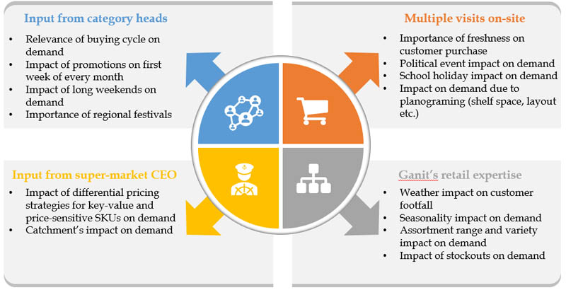
After the store visits, approximately 80 hypotheses on multiple factors were formulated to study their impact on F&V demand. The team performed comprehensive hypotheses testing using techniques like correlation, bivariate and univariate analysis, and statistical significance tests (Student’s t-test, Z tests) to establish the relationship between demand and relevant factors such as festival dates, weather, promotions, and many more.
Data segmentation
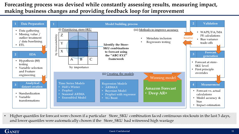
The team emphasized developing a granular model that could accurately forecast a store-SKU combination for each day. A combination of the sales contribution and ease of prediction was built as an ABC-XYZ framework, with ABC indicating the sales contribution (A being the highest) and XYZ indicating the ease of prediction (Z being the lowest). For model building, the first line of focus was on store-SKU combinations that had a high contribution to sales and were the most difficult to predict. This was done to ensure that improving forecasting accuracy has the maximum business impact.
Data treatment
MRL’s transaction data was structured like conventional point of sale data, with fields like mobile number, bill number, item code, store code, date, bill quantity, realized value, and discount value. The team used daily transactional data for the last 2 years for model building. Analyzing historical data helped identity two challenges:
- The presence of numerous missing values
- Some days had extremely high or low sales at bill levels, which indicated the presence of outliers in the data
Missing value treatment
A deep dive into the missing values identified reasons such as no stock available in the store (no supply or not in season) and stores being closed due to planned holiday or external constraints (such as a regional or national shutdown, or construction work). The missing values were replaced with 0, and appropriate regressors or flags were added to the model so the model could learn from this for any such future events.
Outlier treatment
The team treated the outliers at the most granular bill level, which ensured that factors like liquidation, bulk buying (B2B), and bad quality were considered. For example, bill-level treatment may include observing a KPI for each store-SKU combination at a day level, as in the following graph.
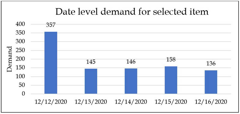
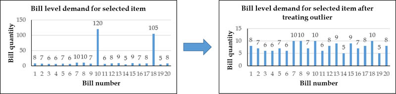
We can then flag dates on which abnormally high quantities are sold as outliers, and dive deeper into those identified outliers. Further analysis shows that these outliers are pre-planned institutional purchases.
These bill-level outliers are then capped with the maximum sales quantity for that date. The following graphs show the difference in bill-level demand.
Forecasting process
The team tested multiple forecasting techniques like time series models, regression-based models, and deep learning models before choosing Forecast. The primary reason for choosing Forecast was the difference in performance when comparing forecast accuracies in the XY bucket against the Z bucket, which was the most difficult to predict. Although most conventional techniques provided higher accuracies in the XY bucket, only the ML algorithms in Forecast provided a 10% incremental accuracy compared to other models. This was primarily due to Forecast’s ability to learn other SKUs (XY) patterns and apply those learnings to highly volatile items in the Z bucket. Through AutoML, the Forecast DeepAR+ algorithm was the winner and chosen as the forecast model.
Iterating to further improve forecasting accuracy
After the team identified Deep AR+ as the winning algorithm, they ran several experiments with additional features to further improve accuracy. They performed multiple iterations on a smaller sample set with different combinations like pure target time series data (with and without outlier treatment), regressors like festivals or store closures, and store-item metadata (store-item hierarchy) to understand the best combination for improving forecast accuracy. The combination of outlier treated target time series along with store-item metadata and regressors returned the highest accuracy. This was scaled back to the original set of 6,230 store-SKU combinations to get the final forecast.

Order quantity calculation
After the team developed the forecasting model, the immediate next step was to use this to decide how much inventory to buy and place orders. Order generation is influenced by forecasted demand, current stock on hand, and other relevant in-store factors.
The following formula served as the basis for designing the order construct.
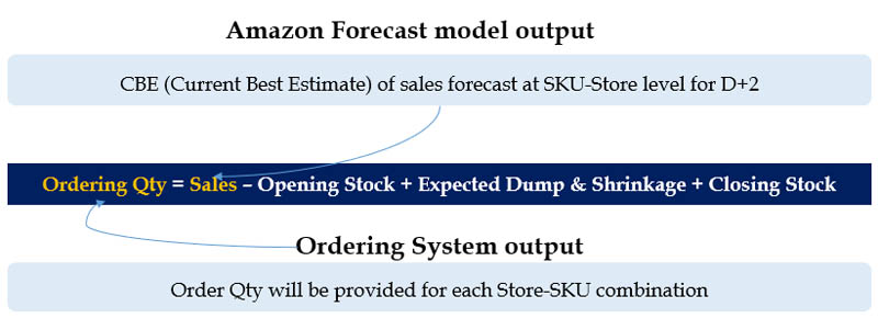
The team also considered other indent adjustment parameters for the automatic ordering system, such as minimum order quantity, service unit factor, minimum closing stock, minimum display stock (based on planogram), and fill rate adjustment, thereby bridging the gap between machine and human intelligence.
Balance under-forecast and over-forecast scenarios
To optimize the output cost of shrinkage with the cost of stockouts and lost sales, the team used the quantiles feature of Forecast to move the forecast response from the model.
In the model design, three forecasts were generated at p40, p50, and p60 quantiles, with p50 being the base quantile. The selection of quantiles was programmed to be based on stockouts and wastage in stores in the recent past. For example, higher quantiles were automatically chosen if a particular store-SKU combination faced continuous stockouts in the last 3 days, and lower quantiles were automatically chosen if the store-SKU had witnessed high wastage. The quantum of increasing and decreasing quantiles was based on the magnitude of stockout or shrinkage within the store.
Automated order placement through Oracle ERP
MRL deployed Forecast and the indent ordering systems in production by integrating them with Oracle’s ERP system, which MRL uses for order placements. The following diagram illustrates the final architecture.
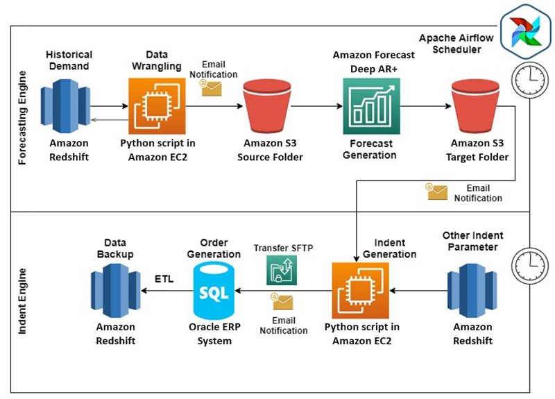
To deploy the ordering system into production, all MRL data was migrated into AWS. The team set up ETL jobs to move live tables to Amazon Redshift (data warehouse for business intelligence work), so Amazon Redshift became the single source of input for future all data processing.
The entire data architecture was divided into two parts:
- Forecasting engine:
- Used historical demand data (1-day demand lag) present in Amazon Redshift
- Other regressor inputs like last bill time, price, and festivals were maintained in Amazon Redshift
- An Amazon Elastic Compute Cloud (Amazon EC2) instance was set up with customized Python scripts to wrangle transaction, regressors, and other metadata
- Post-data wrangling, the data was moved to an Amazon Simple Storage Service (Amazon S3) bucket to generate forecasts (T+2 forecasts for all store-SKU combinations)
- The final forecast output was stored in a separate folder in an S3 bucket
- Order (indent) engine:
- All data required to convert forecasts into orders (such as stock on hand, received to store quantity, last 2 days of orders placed to receive, service unit factor, and planogram-based minimum opening and closing stock) was stored and maintained in Amazon Redshift
- Order quantity was calculated through Python scripts run on EC2 instances
- Orders were then moved to Oracle’s ERP system, which placed an order to vendors
The entire ordering system was decoupled into multiple key segments. The team set up Apache Airflow’s scheduler email notifications for each process to notify respective stakeholders upon successful completion or failure, so that they could take immediate action. The orders placed through the ERP system were then moved to Amazon Redshift tables for calculating the next days’ orders. The ease of integration between AWS and ERP systems led to a complete end-to-end automated ordering system with zero human intervention.
Conclusion
An ML-based approach unlocked the true power of data for MRL. With Forecast, we created two national models for different store formats, as opposed to over 1,000 traditional models that we had been using.
Forecast also learns across time series. ML algorithms within Forecast enable cross-learning between store-SKU combinations, which helps improve forecast accuracies.
Additionally, Forecast allows you to add related time series and item metadata, such as customers who send demand signals based on the mix of items in their basket. Forecast considers all the incoming demand information and arrives at a single model. Unlike conventional models, where the addition of variables leads to overfitting, Forecast enriches the model, providing accurate forecasts based on business context. MRL gained the ability to categorize products based on factors like shelf life, promotions, price, type of stores, affluent cluster, competitive store, and stores throughput. We recommend that you try Amazon Forecast to improve your supply chain operations. You can learn more about Amazon Forecast here. To learn more about Ganit and our solutions, reach out at info@ganitinc.com to learn more.
The content and opinions in this post are those of the third-party author and AWS is not responsible for the content or accuracy of this post.
About the Authors
 Supratim Banerjee is the Chief Transformational Officer at More Retail Limited. He is an experienced professional with a demonstrated history of working in the venture capital and private equity industries. He was a consultant with KPMG and worked with organizations like A.T. Kearney and India Equity Partners. He holds an MBA focused on Finance, General from Indian School of Business, Hyderabad.
 Shivaprasad KT is the Co-Founder & CEO at Ganit Inc. He has a 17+ years of experience in delivering top-line and bottom-line impact using data science in the US, Australia, Asia, and India. He has advised CXOs at companies like Walmart, Sam’s Club, Pfizer, Staples, Coles, Lenovo, and Citibank. He holds an MBA from SP Jain, Mumbai, and a bachelor’s degree in Engineering from NITK Surathkal.
 Gaurav H Kankaria is the Senior Data Scientist at Ganit Inc. He has over 6 years of experience in designing and implementing solutions to help organizations in retail, CPG, and BFSI domains make data-driven decisions. He holds a bachelor’s degree from VIT University, Vellore.