Allocate shared Amazon MSK costs to Kafka topics for cost visibility

Your AWS bill shows Amazon Managed Streaming for Apache Kafka (Amazon MSK) charges at the cluster level, with one cost line item for each cluster. If your organization runs one cluster for several teams, and each team owns its own Kafka topics, you need a way to show each team its share of the spend. This post shows how you can produce that per-topic cost view by combining cluster-level billing data with per-topic usage metrics. The result gives each team a usage-based picture of what it consumes.

Bringing cost and usage together

You can use Amazon MSK to run Apache Kafka at scale while AWS manages the underlying infrastructure, so you can focus on configuring and operating your applications. Many organizations consolidate multiple workloads onto a single cluster, where each team or application owns a set of Kafka topics. Consolidation can help you improve operational efficiency. When you implement per-topic cost visibility, you can show each team its share of the cluster spend.

Producing that view draws on two sources of data, and the solution brings them together.

Cost: cluster-level billing in the CUR

You can locate MSK charges in your AWS Cost and Usage Report (CUR) by cluster ARN and see operations such as RunBroker, RunVolume, and Bandwidth. You use this cluster-level cost as the starting point when you allocate costs to your topics.

Usage: per-topic metrics without cost context

Amazon MSK surfaces per-topic throughput metrics, which provide the usage signal you use to distribute cluster cost across topics. You can use the cluster name that Amazon MSK provides with these metrics. Map that name to the cluster ARN to join usage with billing and produce per-topic cost.

Solution overview

Option A – Enhanced Monitoring: Uses per-topic Amazon CloudWatch metrics published by Amazon MSK.

Option B – Open Monitoring with Amazon Managed Service for Prometheus: A cost-optimized alternative. This option uses the MSK Open Monitoring endpoint at no additional charge and keeps metric cost growth low as topic count grows.

Both options use the same allocation logic and output. Switch between them with one configuration value.

The pipeline runs in five steps:

1. Read cluster cost from CUR – A daily AWS Lambda function reads MSK line items by cluster ARN and day.
2. Bridge identifiers – The function calls ListClustersV2 to map cluster name to ARN.
3. Read per-topic usage – The function retrieves each topic’s daily throughput. This step differs between Option A and Option B.
4. Allocate proportionally – For each day, the function distributes that day’s cluster cost across topics based on each topic’s share of throughput.
5. Publish results – The function writes allocation data as Apache Parquet to Amazon Simple Storage Service (Amazon S3) and refreshes an Amazon Athena table. You visualize the results in AWS Quick Sight.

The following diagram shows the pipeline.

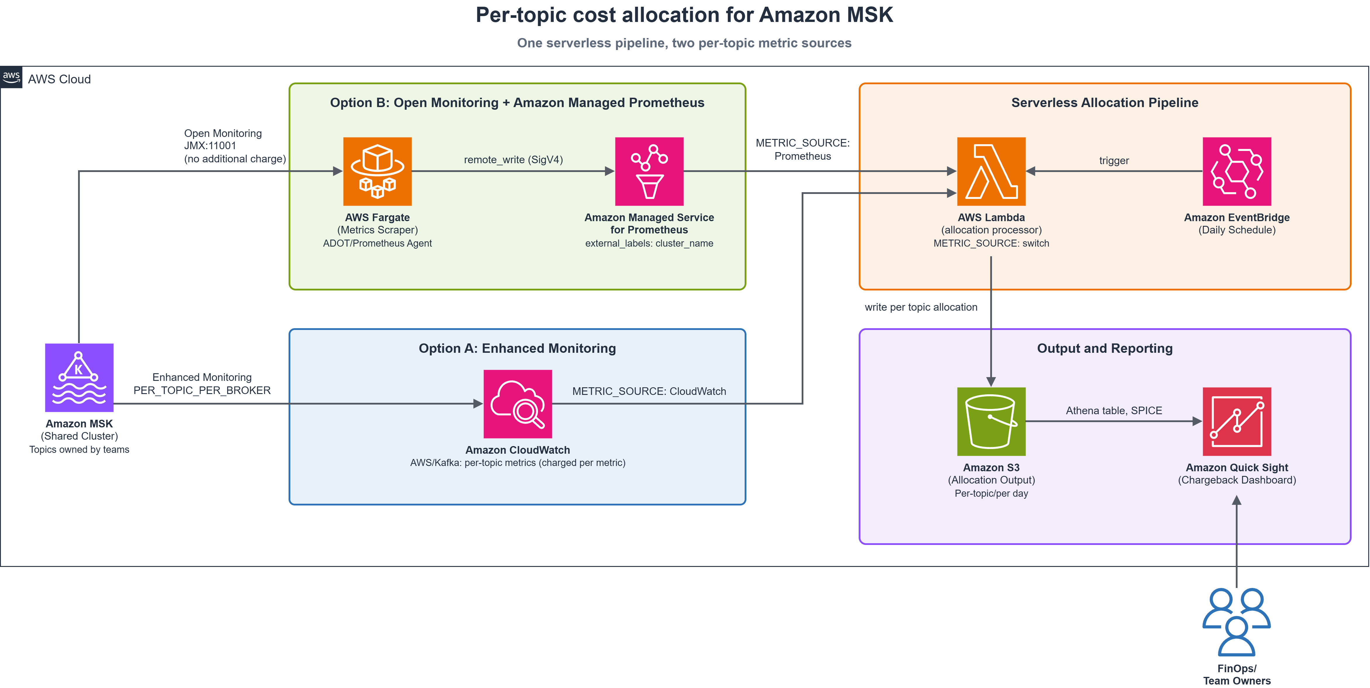
Figure 1: Solution architecture. A single serverless pipeline supports both per-topic metric sources, selected with the METRIC_SOURCE environment variable

How the allocation works

For each cluster and day, the function computes each topic’s share of ingress bytes and applies that share to the cost:

topic_run_cost = day_broker_cost × (topic_bytes / total_cluster_bytes)
topic_storage_cost = day_storage_cost × (topic_bytes / total_cluster_bytes)
topic_total_cost = topic_run_cost + topic_storage_cost

The function assigns 30 percent of the cost to a topic that carries 30 percent of ingress. Allocations always sum to the day’s total. During a partial outage, the function distributes costs only among topics for which you have configured metrics.

Two behaviors to know:

• Idle topics get no row. If only 3 of 20 report traffic, those 3 absorb the full cost. The allocation_method column catches this.
• If no topic reports traffic for a cluster-day, the function falls back to an even split across all topics you have configured.

Why bytes-in as the allocation weight

Bytes-in is available from both metric sources and correlates well with broker compute and network cost.

However, bytes-in is a proxy. Its limitations:

• It can’t see retention. Two topics with identical throughput but different retention periods use different storage.
• It can’t see replication factor or compression, which change actual bytes on disk.
• It can’t see consumer fan-out. A topic read by ten consumer groups looks the same as one read by one.

Other factors can drive your costs, such as egress (consumer read volume), partition count, or storage retention. In that case, you can adapt the same pipeline to use a different allocation weight or a blended model.

Report unallocated charges (data transfer, tiered storage, MSK Connect) explicitly so finance has a more complete picture.

Prerequisites

Before you begin, make sure you have:

• An active Amazon MSK Provisioned cluster with topics carrying traffic. (Amazon MSK Serverless is out of scope. It bills differently and does not expose per-topic BytesInPerSec.)
• AWS CUR (or AWS Data Exports for CUR 2.0) delivering Parquet to Amazon S3 with resource IDs enabled. Uses CUR 2.0 snake_case column names.
• An AWS Glue catalog table over the CUR data with correct partition configuration.
• Permissions to create AWS Lambda functions, IAM roles, Athena tables, and Quick Sight resources.
• Quick Sight Enterprise edition (for SPICE datasets and row-level security in the reporting layer).
• For Option B only: a private subnet in the MSK virtual private cloud (VPC) for the scraper, and an Amazon Managed Service for Prometheus workspace.

Timing: CUR lags up to 24 hours. Per-topic metrics exist only from the moment you enable them.

Sourcing per-topic usage: Two options

How you collect per-topic usage is the main design decision in this solution, because it determines your monitoring cost and setup effort. The pipeline supports both options, and you select one with the METRIC_SOURCE environment variable.

Option A (recommended starting point): Enhanced Monitoring

When you set Enhanced Monitoring to PER_TOPIC_PER_BROKER, MSK publishes per-topic throughput metrics to CloudWatch. The Lambda function aggregates each topic’s daily usage with GetMetricStatistics calls.

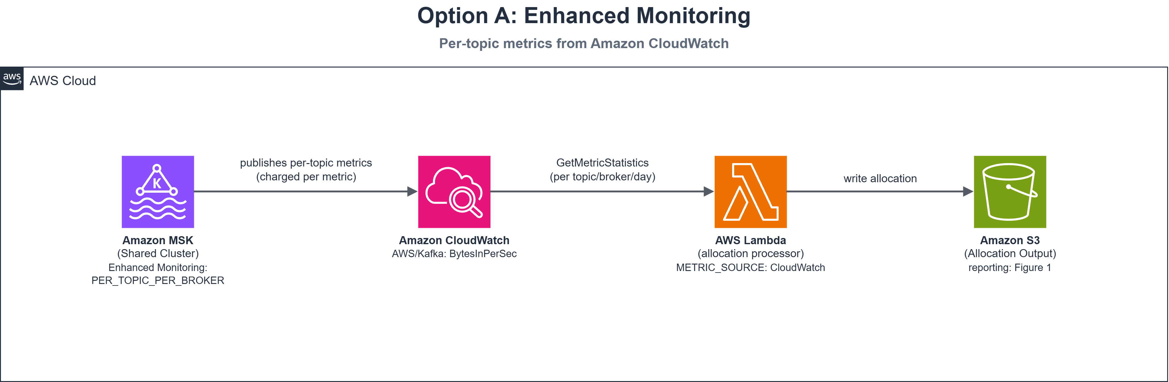
Figure 2: Option A collection path. Amazon MSK publishes per-topic metrics to CloudWatch, and the allocation function reads them directly

Code sample — reading per-topic metrics from CloudWatch:

result = cloudwatch.get_metric_statistics(
    Namespace='AWS/Kafka', MetricName='BytesInPerSec',
    Dimensions=[
        {'Name': 'Cluster Name', 'Value': cluster_name},
        {'Name': 'Broker ID', 'Value': str(broker_id)},
        {'Name': 'Topic', 'Value': topic},
    ],
    StartTime=day_start, EndTime=day_end,
    Period=86400, Statistics=['Sum'],
)

Note: BytesInPerSec is a rate. Period=86400 with Statistics=[Sum] returns a valid relative weight for proportional allocation, not total bytes.

Why start here: Nothing to deploy. Change one cluster setting and metrics appear in CloudWatch.

The trade-off: CloudWatch bills per metric. PER_TOPIC_PER_BROKER publishes a metric set for every topic-broker pair, so cost grows with both.

Scaling tip: At scale (over 50 clusters, over 200 topics), switch to GetMetricData (up to 500 metrics per call) instead of iterating GetMetricStatistics.

Option B (cost-optimized): Open Monitoring with Amazon Managed Service for Prometheus

Kafka brokers expose operational metrics through Java Management Extensions (JMX). Amazon MSK Open Monitoring makes these infrastructure metrics available in Prometheus format on port 11001 at no cost.

You run a scraper (AWS Fargate with an AWS Distro for OpenTelemetry (ADOT) Collector) that forwards metrics to a Prometheus workspace through SigV4 remote write. The task role needs the aps:RemoteWrite permission.

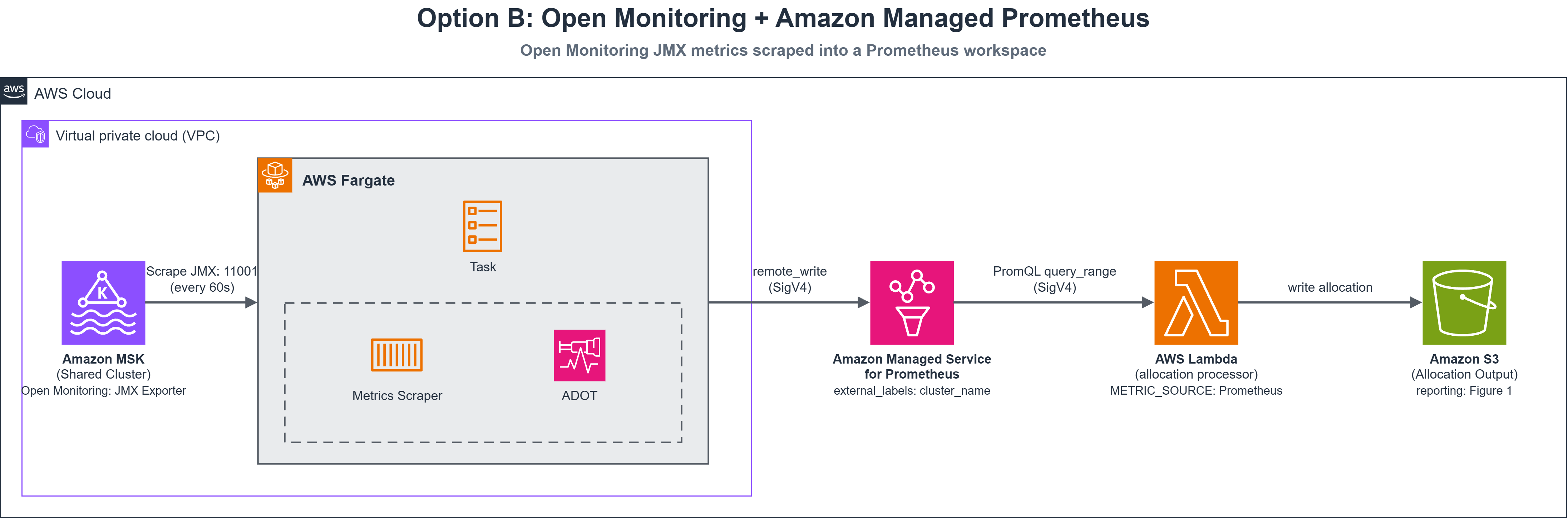
Figure 3: Option B collection path. A VPC scraper collects JMX metrics at no additional charge and forwards them to Prometheus

Scraper configuration (Prometheus agent):

global:
  scrape_interval: 60s
  external_labels:
    cluster_name: "<your-cluster-name>"  # allocation query filters on this

scrape_configs:
  - job_name: msk-jmx
    metrics_path: /metrics
    static_configs:
      - targets:
          - "b-1.<cluster>.<id>.kafka.<region>.amazonaws.com:11001"
          - "b-2.<cluster>.<id>.kafka.<region>.amazonaws.com:11001"

remote_write:
  - url: https://aps-workspaces.<region>.amazonaws.com/workspaces/<workspace-id>/api/v1/remote_write
    sigv4:
      region: <region>
      role_arn: arn:aws:iam::<central-account-id>:role/MskPromRemoteWriteRole
    queue_config:
      capacity: 2500
      max_samples_per_send: 1000

Get broker hostnames from GetBootstrapBrokers. For dynamic lists, use Prometheus file_sd_configs.

PromQL query for per-topic usage:

sum by (topic) (
  avg_over_time(
    kafka_server_BrokerTopicMetrics_OneMinuteRate_BytesInPerSec{cluster_name="<cluster>"}[1d]
  )
) * 86400

This averages broker rates over 24 hours into one value per topic, producing a comparable weight.

Open Monitoring is available at no additional charge and the Prometheus workspace bills on samples ingested, so metric cost grows slowly. This suits large fleets.

How the function discovers topics

The function resolves topic lists through a tiered lookup:

1. Static topic map – An environment variable holding JSON keyed by cluster name. No API calls needed. Works well when you already track topic ownership in config or infrastructure code.
2. Amazon MSK ListTopics API – Control-plane call, no VPC connectivity needed.
3. CloudWatch ListMetrics – Reads topics from metric dimensions (Enhanced Monitoring only).
4. Previous allocation output – Falls back to yesterday’s topic list from S3.

The tiered lookup keeps the function working whether or not Enhanced Monitoring is enabled:

def discover_topics(cluster_name, kafka_client=None, cluster_arn=None):
    """Resolve the topic list without requiring Enhanced Monitoring.
    Tiers are tried in order; the first that returns topics wins."""
    # Tier 1: static map from an env var (no API calls). Set TOPIC_LIST_JSON
    # to a JSON object keyed by cluster name, e.g. {"<cluster>": ["<topic>", ...]}
    if TOPIC_LIST_JSON:
        mapping = json.loads(TOPIC_LIST_JSON)
        if cluster_name in mapping:
            return set(mapping[cluster_name])
    # Tier 2: MSK ListTopics API - works at DEFAULT monitoring, no extra cost
    if kafka_client and cluster_arn:
        topics = _discover_topics_via_msk_api(kafka_client, cluster_arn)
        if topics:
            return topics
    # Tier 3: CloudWatch ListMetrics - only returns topics when Enhanced
    # Monitoring (PER_TOPIC_PER_BROKER) is enabled
    topics = _discover_topics_via_cloudwatch(cluster_name)
    if topics:
        return topics
    # Tier 4: fall back to the topic list from yesterday's allocation output in S3
    return _topics_from_previous_allocations()

Choosing between the options

For steady topics, both options typically produce comparable results. The choice is cost and operating model:

Note: Figures are illustrative, not AWS list prices. Recalculate using the CloudWatch, Prometheus, and Fargate pricing pages.

Guideline: if monitoring cost is below 5 percent of MSK spend, take Option A. Above 10 percent, Option B repays the setup quickly.

You can enable Enhanced Monitoring only on clusters where chargeback accuracy matters, and switch to Option B later with one environment variable change.

Deploying the allocation pipeline

Deploy with AWS Cloud Development Kit (AWS CDK). The core Lambda function (Python 3.11, 1 GB, 10-min timeout) uses the AWS SDK for pandas layer for Parquet processing. Two triggers invoke the function, for resilience:

• An Amazon S3 event notification fires when a new CUR Parquet file arrives, so allocation runs as soon as fresh cost data lands.
• An Amazon EventBridge rule runs daily at 06:00 UTC as a fallback, in case the S3 event doesn’t arrive or CUR delivery lags.

Set METRIC_SOURCE to cloudwatch for Option A or prometheus for Option B. For Option B, you also supply the workspace query endpoint and label names.

The handler at a glance

The following handler function orchestrates the five-step pipeline. Each step delegates to a dedicated function, described in the sections that follow.

def handler(event, context):
    """Lambda entry point --- runs the five-step pipeline once per invocation."""
    # Step 1: read cluster cost from CUR (MSK rows only)
    daily_cur = read_cur_costs_via_athena()
    if not daily_cur:
        return _resp(200, 'No MSK costs found in CUR data')
    # Step 2: bridge identifiers - group cluster ARNs by account
    clusters_by_account = _group_clusters_by_account(daily_cur)
    # Steps 3-4: read per-topic usage and allocate cost proportionally, per cluster
    all_rows, errors = [], []
    for account_id, cluster_arns in clusters_by_account.items():
        try:
            all_rows.extend(process_account(account_id, cluster_arns, daily_cur))
        except Exception as e:
            errors.append({'account': account_id, 'error': str(e)})
    # Step 5: publish results - write Parquet to S3, refresh the Athena table
    write_allocations(all_rows)
    refresh_allocation_table()
    return _resp(200, {'rows_written': len(all_rows), 'errors': len(errors)})

CDK stack – Lambda function definition:

allocation_fn = lambda_.Function(
    self, "AllocationProcessor",
    runtime=lambda_.Runtime.PYTHON_3_11,
    handler="handler.handler",
    code=lambda_.Code.from_asset("src/lambda/allocation_processor"),
    timeout=Duration.minutes(10),
    memory_size=1024,
    dead_letter_queue=dlq,
    environment={
        "OUTPUT_BUCKET": allocation_bucket.bucket_name,
        "ATHENA_DATABASE": cur_database_name,
        "CUR_TABLE_NAME": cur_table_name,
        "ATHENA_OUTPUT": f"s3://{allocation_bucket.bucket_name}/athena-results/",
        # Option A. Switch to "prometheus" for Option B.
        "METRIC_SOURCE": "cloudwatch",
        # Option B only:
        # "AMP_QUERY_URL": "https://aps-workspaces.<region>.amazonaws.com/"
        # "workspaces/<workspace-id>/api/v1",
        # "AMP_CLUSTER_LABEL": "cluster_name",
        # "AMP_TOPIC_LABEL": "topic",
    },
    layers=[pandas_layer],
)

Triggers:

# Trigger 1: process when new CUR data arrives
cur_bucket.add_event_notification(
    s3.EventType.OBJECT_CREATED,
    s3n.LambdaDestination(allocation_fn),
    s3.NotificationKeyFilter(prefix="cur-clean/", suffix=".parquet"),
)

# Trigger 2: daily schedule as fallback
daily_rule = events.Rule(
    self, "DailyAllocationRule",
    schedule=events.Schedule.cron(hour="6", minute="0"),
)
daily_rule.add_target(targets.LambdaFunction(allocation_fn))

The stack provisions an Amazon Simple Queue Service (Amazon SQS) dead-letter queue with 14-day retention for failed invocations, Amazon Simple Notification Service (Amazon SNS) alerts, and CloudWatch alarms. To subscribe your team, add sns.Topic.add_subscription(subscriptions.EmailSubscription("your-dl@example.com")) in CDK, or subscribe manually through the Amazon SNS console.

The stack creates the AWS Glue table over the allocation output, so you don’t need to write DDL by hand. Deploy it with:

cdk bootstrap  # once per account and Region
cdk deploy

Invoke the function once manually to produce a first allocation.

Reading CUR efficiently at scale

The function queries CUR through Amazon Athena to get only MSK rows. Filter on partition columns so Athena prunes whole partitions:

SELECT line_item_resource_id, line_item_usage_start_date,
       line_item_unblended_cost, line_item_operation
FROM "<cur_database>"."<cur_table>"
WHERE billing_period IN ('<current_month>', '<previous_month>')
  AND line_item_product_code = 'AmazonMSK'
  AND line_item_resource_id LIKE 'arn:aws:kafka:%'
  AND line_item_usage_start_date >= TIMESTAMP '<start_of_prev_month>'
  AND line_item_unblended_cost != 0

The query reads two months because AWS can update CUR line items after the first delivery. Adjust arn:aws:kafka: for GovCloud or the China Regions.

Publishing and querying the results

The function writes allocation results to Amazon S3 as Snappy-compressed Parquet, partitioned by billing period. Each row covers one topic on one day with cluster identity, usage weight, and allocated cost.

Each run overwrites the file for its billing period. This helps prevent double-counting on CUR redeliveries.

Output schema:

Verifying the numbers

Run this reconciliation query before publishing a dashboard. Schedule it as a Lambda post-step with an AllocationVariance CloudWatch alarm:

SELECT allocation_date,
       cluster_name,
       SUM(total_cost) AS allocated,
       MAX(cluster_run_cost_day + cluster_storage_cost_day) AS billed,
       SUM(total_cost) - MAX(cluster_run_cost_day + cluster_storage_cost_day) AS variance,
       MAX(allocation_method) AS method,
       COUNT(*) AS topics_charged
FROM topic_cost_allocation
WHERE billing_period = '<YYYY-MM>'
GROUP BY allocation_date, cluster_name
HAVING ABS(SUM(total_cost)
    - MAX(cluster_run_cost_day + cluster_storage_cost_day)) > 0.01
ORDER BY allocation_date;

An empty result means allocations reconcile. Rows indicate days where topic discovery and cost data disagreed.

Mapping topics to teams

The function derives owners from topic naming conventions. Pass an explicit topic-to-team map where conventions fail. Unmapped topics appear as unfamiliar owners.

Visualizing cost by topic in Quick Sight

Create an Athena data source in Quick Sight, import into SPICE, and schedule daily refreshes.

A useful dashboard typically includes:

• A detail table of cost by team, topic, and month.
• A bar chart of total cost by topic.
• Filter controls for cluster, topic, and time period.

Apply Quick Sight row-level security against client_id so teams see only their own numbers. Row-level security requires Enterprise edition.

Extending to multiple accounts

The pipeline extends to multi-account setups:

• The central account reads the consolidated CUR.
• The Lambda function assumes a read-only role in each member account (by using AWS Security Token Service (AWS STS)) to list clusters and read usage, writing one consolidated dataset.
• For Option B, a single central Prometheus workspace receives remote-writes from every member account’s scraper, each stamping its own cluster_name label.

One dataset and one dashboard across all accounts.

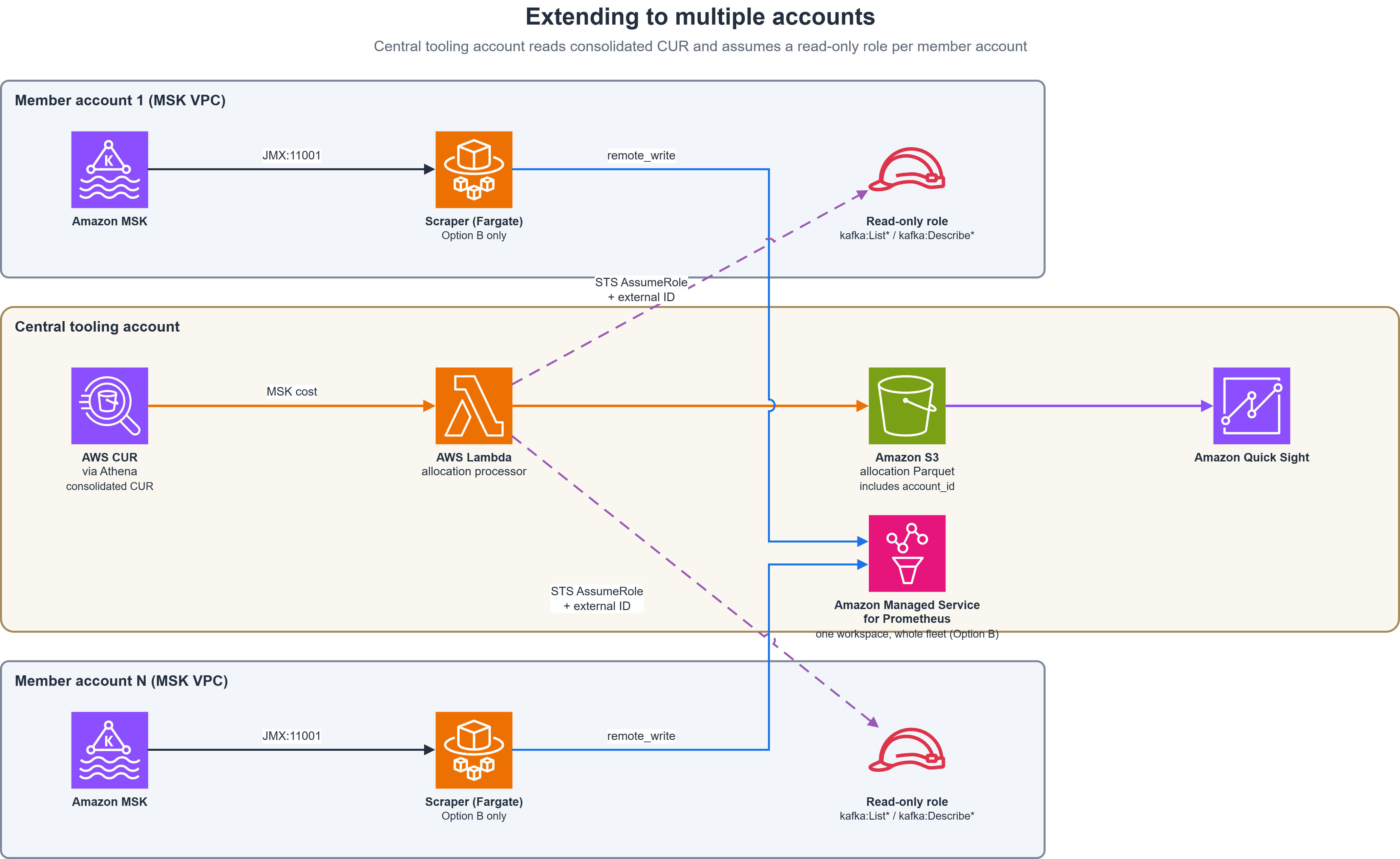
Figure 4: Multi-account extension. The central tooling account owns the pipeline and reaches into member accounts through a scoped, read-only role

Security considerations

This pipeline reads billing data and crosses account boundaries.

Grant the central execution role only the permissions it needs to: read the CUR and Glue catalog, run Athena queries, write to the allocation S3 bucket, and assume member-account roles.

Member-account role is read-only. Require a shared external ID on every AssumeRole call to help mitigate the confused-deputy problem.

For Option B, restrict port 11001 to the scraper’s security group. Consider AWS PrivateLink for remote write.

Encrypt CUR, allocation output, and Athena results at rest using SSE-KMS (recommended for financial data). Use TLS to encrypt data in transit, including the scraper’s remote write and Athena connections.

The output reveals what every team spends. Treat the output bucket and Quick Sight dataset as financial reports.

Cost of running the solution

The pipeline itself is inexpensive (Lambda, Athena, S3, Amazon EventBridge are negligible). Two items dominate:

• The metric source: ~$90 (Option A) compared to ~$11 (Option B) per month on the example cluster.
• Quick Sight user licenses: frequently the largest cost, scaling with how many people get access.

Clean up

To avoid ongoing charges, remove the resources you created. Delete Athena query result files and the CUR delivery configuration if created solely for this solution.

cdk destroy

If you enabled Enhanced Monitoring solely for this solution, return to the previous level. For Option B, remove the scraper and Prometheus workspace.

Conclusion

This pipeline bridges cluster-level CUR cost to topic-level usage, giving each team visibility into its share of the spend. Switch between monitoring options with one environment variable. Pick a cluster and run the allocation to get started.

Learn more:

• Monitoring an Amazon MSK cluster – For monitoring levels and Open Monitoring setup.
• Amazon Managed Service for Prometheus – For workspace configuration and ingestion.
• Querying Cost and Usage Reports using Amazon Athena – For CUR table setup.
• Using Amazon Athena data with Quick Sight – For the reporting layer.

About the authors