Artificial Intelligence
Amazon SageMaker Ground Truth: Using A Pre-Trained Model for Faster Data Labeling
With Amazon SageMaker Ground Truth, you can build highly accurate training datasets for machine learning quickly. SageMaker Ground Truth offers easy access to public and private human labelers and provides them with built-in workflows and interfaces for common labeling tasks. Additionally, SageMaker Ground Truth can lower your labeling costs by up to 70% using automatic labeling, which works by training Ground Truth from data labeled by humans so that the service learns to label data independently. This previous blog post explains how automated data labeling works and how to evaluate its results.
What you may not know is that SageMaker Ground Truth trains models for you over the course of a labeling job, and that these models are available for use after a labeling job concludes! In this blog post, we will explain how you can use a model trained from a previous labeling job to “jump start” a subsequent labeling job. This is an advanced feature, only available through the SageMaker Ground Truth API.
| About this blog post | |
| Time to read | 30 minutes |
| Time to complete | 8 hours |
| Cost to complete | Under $600 |
| Learning level | Intermediate (200) |
| AWS services | Amazon SageMaker, Amazon SageMaker GroundTruth |
This post builds on the following prior post – you may find it useful to review it first:
As part of this blog, we will create three different labeling jobs, as described below.
- An initial labeling job with the “auto labeling” feature enabled. At the end of this labeling job, we will have a trained machine learning model capable of making high quality predictions on the sample dataset.
- A subsequent labeling job with a different set of images drawn from the same dataset as the first labeling job. In this labeling job, the machine learning model that was produced as an output of the first labeling job will be provided to accelerate the labeling process
- A repetition of the second labeling job, but without the pre-trained machine learning model. This labeling job is intended to serve as a control to demonstrate the benefit of using the pre-trained model.
We will use an Amazon SageMaker Jupyter notebook that uses the API to produce bounding box labels for our dataset.
To access the demo notebook, start an Amazon SageMaker notebook instance using an ml.m4.xlarge instance type. You can follow this step-by-step tutorial to set up an instance. On Step 3, make sure to mark “Any S3 bucket” when you create the IAM role! Open the Jupyter notebook, choose the SageMaker Examples tab, and launch object_detection_pretrained_model.ipynb.
Prepare Datasets
Let’s prepare our dataset to be used in creating our labeling jobs. We will create two sets of 1250 images from this dataset. We will use the first batch in our initial labeling job and the other batch for our two subsequent jobs, one with the pre-trained model and one without.
Next, run all the cells under ‘Prepare Dataset’ in the demo notebook. Running these cells will perform the following steps.
- Get the full collection of 2500 images from the dataset repository.
- Divide the dataset in two batches of 1250 images each.
Create An Initial Labeling Job With Active Learning
Now let’s run our first job. Run all of the cells under the “Iteration #1: Create Initial Labeling Job” heading of the notebook. You need to modify some of the cells, so read the notebook instructions carefully. Running these sections will perform the following steps.
- Prepare the first set of 1250 from the previous step for use in our first labeling job.
- Create labeling instructions for an object detection labeling job.
- Create an object detection labeling job request.
- Submit the labeling job request to SageMaker Ground Truth.
The job should take about four hours. When it’s done, run all of the cells in the “Analyze Initial Active Learning labeling job results” sections. These sections will produce a wealth of information that will help you understand the labeling job that you performed. In particular, we can see that the total cost was $217.18, of which 78% was attributable to the costs of manual labeling by the public work team. It’s worth pointing out that even at this stage there is modest cost savings due to our use of auto labeling – without it, the labeling cost would have been $235. In general, larger datasets (on the order of multiple thousands of objects) will be able to leverage greater use of auto labeling. In the rest of this blog, we will seek to improve the auto labeling performance even on this small 1,250-object dataset through the use of a pre-trained model.
In a previous blog post “Annotate data for less with Amazon SageMaker Ground Truth and automated data labeling” we described the batch-wise nature of a labeling job. In this blog post, we again refer to the batch-by-batch statistics of our labeling job. The plots below show that the model did not begin auto-labeling images until the 4th iteration. In the end, the ML model was able to annotate a little less than half of the entire dataset. We will look to increase the share of machine labeled data and consequently decrease the overall cost by using a pre-trained model in the next step.
Verify that the cell titled “Wait for Completion of Job” returns the job status “Completed” before proceeding to the next step.
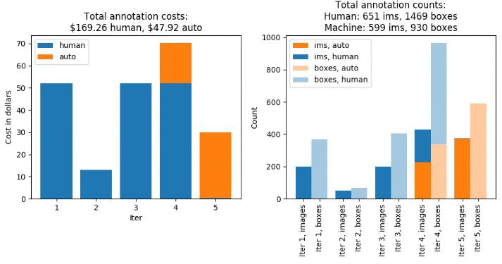
Figure 1. Labeling costs and metrics for the initial labeling job.
Create A Second Labeling Job With A Pre-Trained Model
Now that the first labeling job is complete, we’ll prepare the second labeling job. We’ll reuse much of the original labeling job request, but we’ll need to specify the pre-trained machine learning model. We can query the original labeling job to get the Amazon ARN for the final machine learning model trained during the first job.
We’ll use this for the InitialActiveLearningModelArn parameter in the labeling job request.
In the demo notebook, run all the cells under the “Iteration #2: Labeling Job with Pre-Trained Model” heading. Running these sections will perform the following steps.
- Create an object detection labeling job request in which the model trained in the previous labeling job is provided.
- Submit the labeling job request to Ground Truth.
The job should take about four hours. When it’s done, run all of the cells in the “Analyze Active Learning labeling job with pre-trained model results” sections. This will produce a wealth of information similar to what we saw after the previous labeling job. You should already see some key differences in the number of machine-labeled dataset objects! In particular, the machine learning model is able to start labeling data in the third iteration, and when it does, it annotates almost the entire remainder of the dataset! Note that the cost associated with manual labeling is much lower than before. Although the cost associated with auto labeling has increased, this increase is smaller in magnitude than the decrease in the human labeling cost. Consequently, the overall cost of this labeling job – $146.80 – is 33% lower than that of the first labeling job.
Verify that the cell titled “Wait for Completion of Job” returns the job status “Completed” before proceeding to the next step.
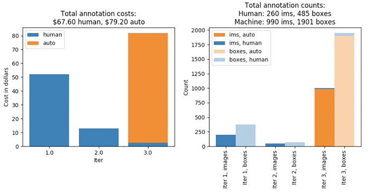
Figure 2. Labeling costs and metrics for the second labeling job with the use of a pre-trained model.
Repeat the Second Labeling Job Without the Pre-Trained Model
In the previous labeling job, we saw a substantial improvement in run time and the number of machine labeled dataset objects relative to the first dataset. However, one may naturally ask how much of the difference is due to the difference in the underlying data. Although both datasets have the same labels and are sampled from the same, larger dataset, a controlled study will provide a fairer assessment. To that end, we’ll now repeat the second labeling job with all the same settings, but remove the pre-trained model. In the demo notebook, run all the cells in the “Labeling Job without Pre-trained model”. Running these sections will perform the following steps.
- Duplicate the labeling job request from the second labeling job with the removal of the pre-trained model.
- Submit the labeling job request to Ground Truth
The job should take about four hours. When it’s done, run all of the cells under the “Iteration #3: Second Data Subset Without Pre-Trained Model” heading. Again, this will produce plots that look similar to those generated in the previous steps. However, these figures should look more similar to the results of the first labeling job than the second. Notice that the overall cost is $189.64, and that the job took five iterations to complete. Notice that this is 29% larger than when we used the pre-trained model to help label this data!
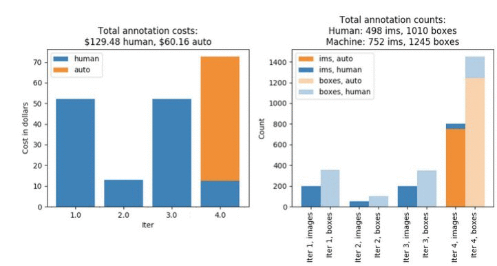
Figure 3. Labeling costs and metrics for the third labeling job, which uses the same dataset as the second labeling job without the benefit of the pre-trained model.
Compare Results
Now that we’ve run all there labeling jobs, we can compare the results more fully. First, consider the left-hand plot shown below. The total elapsed running time for the labeling job that uses the pre-trained model is less than half the time required for the jobs that don’t make use of the pre-trained model. We can also see in the right-hand plot below that this reduction in time goes hand-in-hand with a larger fraction of auto-labeled data. The reason that the labeling job that uses the pre-trained model is so much faster is because the machine learning model does more of the work, which is much more efficient than manual labeling.
It should be noted that some amount of variability is expected in these results. Due to the small random effects introduced by the pool of workers available when these labeling jobs were performed, the small fluctutations that may be seen in training the machine learning model, etc., a repeated trial of these three labeling jobs may result in slightly different numbers. However, the substantial gain in cost and time savings seen in experiment #2 is predominately due to the use of the pre-trained model.

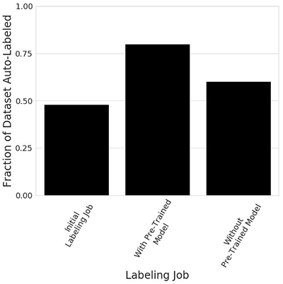
Figure 4. Comparison of labeling time and auto-labeling efficiency across the three labeling jobs.
Finally, the plot below shows that the reduction in labeling time and the increase in the fraction of data annotated by the machine learning model lead to a measurable reduction in the total labeling cost. In this example we see that when labeling the second dataset, using a pre-trained model leads to a 23% reduction in cost relative to the control scenario where the pre-trained model was not used – $146.80 vs $189.64.
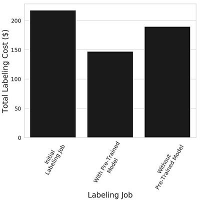
Figure 5. Total labeling cost across the three labeling jobs.
Conclusion
Let’s review what we covered in this exercise.
- We gathered a dataset consisting of 2500 images of birds from the Open Images dataset.
- We split this dataset into two halves.
- We created an object detection labeling job for the first subset of 1250 images and saw that approximately 48% of the dataset was machine-labeled.
- We created a second labeling job for the second subset, and we specified the machine learning model that was trained during the first labeling job. This time we found that approximately 80% of the dataset was machine-labeled.
- As a final benchmark, we re-ran the second labeling job without specifying the pre-trained model. Now we found that approximately 60% of the dataset was machine-labeled.
- In the end, we saw a 50% reduction in time required to acquire labels, and a 23% reduction in total labeling cost when we use a pre-trained model. This is highly context dependent, and results will vary from application to application. However, the workflow illustrated in this example demonstrates the value of using a pre-trained model for successive labeling jobs.
If we were to acquire a new unlabeled dataset in this domain (e.g., object detection for birds), we could setup another labeling job, and specify the model trained in our second labeling job. The use of pre-trained machine learning models thus allows you to run labeling jobs in succession, with each job improving from the predictive ability gained through the previous job. Remember that the pre-trained model capability requires you to use the “job chaining” feature (described in https://aws.amazon.com/blogs/aws/amazon-sagemaker-ground-truth-keeps-simplifying-labeling-workflows/) or to use the Amazon SageMaker Ground Truth API, as we demonstrated in the accompanying example notebook.
About the Authors
 Prateek Jindal is a software development engineer for AWS AI. He is working on solving complex data labeling problems in the machine learning world and has a keen interest in building scalable distributed solutions for his customers. In his free time, he loves to cook, try out new restaurants, and hit the gym.
 Jonathan Buck is a software engineer at Amazon. His focus is on building impactful software services and products to democratize machine learning.