Artificial Intelligence
Annotate data for less with Amazon SageMaker Ground Truth and automated data labeling
With Amazon SageMaker Ground Truth, you can easily and inexpensively build more accurately labeled machine learning datasets. To decrease labeling costs, use Ground Truth machine learning to choose “difficult” images that require human annotation and “easy” images that can be automatically labeled with machine learning. This post explains how automated data labeling works and how to evaluate its results.
Run an object detection job with automated data labeling
In a previous blog post, Julien Simon described how to run a data labeling job using the AWS Management Console. For finer control over the process, you can use the API. To show how, we use an Amazon SageMaker Jupyter notebook that uses the API to produce bounding box annotations for 1000 images of birds.
Note: The cost of running the demo notebook is about $200.
To access the demo notebook, start an Amazon SageMaker notebook instance using an ml.m4.xlarge instance type. You can follow this step-by-step tutorial to set up an instance. On Step 3, make sure to mark “Any S3 bucket” when you create the IAM role! Open the Jupyter notebook, choose the SageMaker Examples tab, and launch object_detection_tutorial.ipynb, as follows.
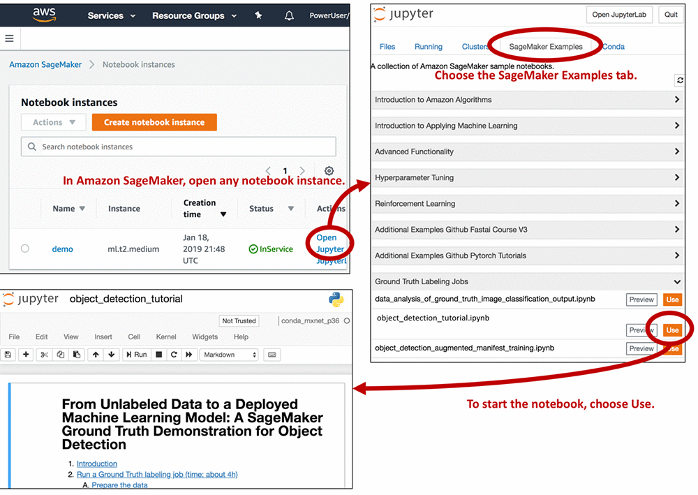
Run all of the cells in the “Introduction” and “Run a Ground Truth labeling job” sections of the notebook. You need to modify some of the cells, so read the notebook instructions carefully. Running these sections:
- Creates a dataset with 1,000 images of birds
- Creates object detection instructions for human annotators
- Creates an object detection annotation job request
- Submits the annotation job request to Ground Truth
The job should take about 4 hours. When it’s done, run all of the cells in the “Analyze Ground Truth labeling job results” and “Compare Ground Truth results to standard labels” sections. This produces a lot of information in plot form. To understand how Ground Truth annotates data, let’s look at some of the plots in detail.
Active learning and automated data labeling
The plots show that annotating the whole dataset took five iterations. In each iteration, Ground Truth sent out a batch of images to Amazon Mechanical Turk annotators. The following graph shows the number of images (abbreviated ‘ims’ in the plot) produced on each iteration and the number of bounding boxes in these images. Your results might differ slightly.
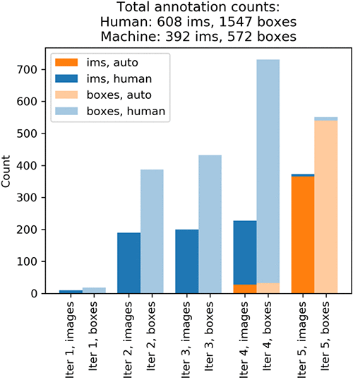
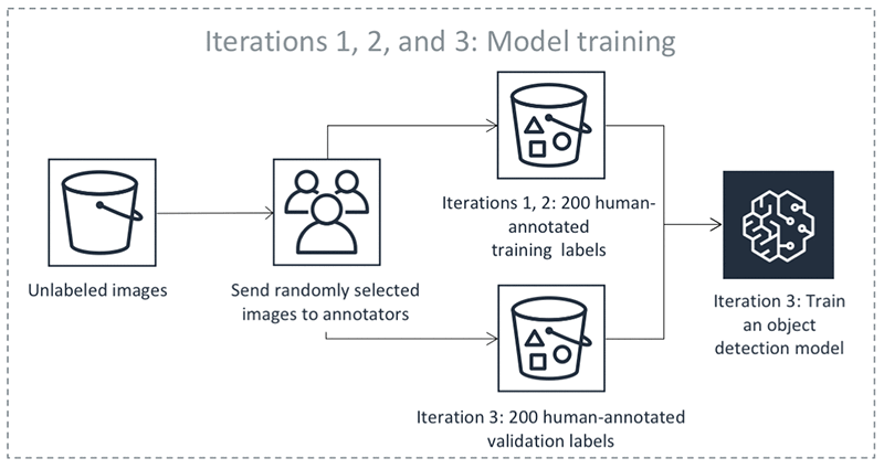
On iteration 1, Mechanical Turk workers annotated a small test batch of 10 randomly chosen images. This batch validates the end-to-end execution of the labeling task. On iteration 2, Mechanical Turk workers annotated another 190 randomly chosen images. This is the validation dataset. It’s used later by a supervised machine learning algorithm to produce automated labels. Iteration 3 created a training dataset by obtaining human-annotated labels on 200 more randomly chosen images. Throughout the process, Ground Truth consolidates each label from multiple human-annotated labels to avoid single-annotator bias. For more information, see the notebook and the Amazon SageMaker Developer Guide.
Now that it has small training and validation datasets, Ground Truth is ready to train the algorithm that later produces automated labels. The following diagram shows the process:
Because automated labeling involves comparing human-annotated labels to labels produced by machine learning, you need to choose a measure of bounding box quality. For this exercise, use the mean Intersection over Union (mIoU). An mIoU of 0 means that there is no overlap between two sets of bounding boxes. A mIoU of 1 means that the two sets of bounding boxes overlap perfectly. Your goal is to produce automated labels that would have an mIoU of at least 0.6 with the human-annotated labels, had you also gotten human annotations on corresponding images. This is slightly higher than 0.5, a threshold commonly used in computer vision to indicate a match between bounding boxes (see for example the “This is a break from tradition…” note here).
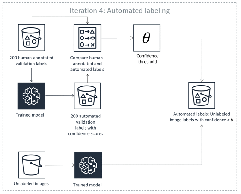
Equipped with a trained DL model and the mIoU measure, Ground Truth is ready to produce the first automated labels on iteration 4. There are four steps:
- Use the machine learning algorithm to predict the bounding boxes and their confidence scores on the validation dataset. Remember that you got human-annotated labels for this dataset on iterations 1 and 2. The algorithm assigns each bounding box a confidence score between 0 and 1. By averaging these scores for a particular image, the algorithm gets an image confidence score that tells you how confident the algorithm is in its prediction.
- For any image confidence threshold, we can compute how well the algorithm’s predictions on images that are scored above the threshold match human-annotated labels. Find a threshold so that the mIoU of above-threshold labels is at least 0.6. Let’s call the resulting threshold θ.
- Use the algorithm to predict bounding boxes and their confidence scores on the remaining unlabeled dataset, which contains 600 images.
- Take any unlabeled dataset predictions whose confidence scores exceed θ. In Steps 1 and 2, we made sure that on the human-annotated validation dataset these confidence scores indicate automated annotations that match human labels well. Now assume that the annotations also match what human annotators would have produced on unlabeled data. Ground Truth keeps these annotations as automated labels produced by the algorithm. There may be no need to send the images with automated labels with a high confidence score to human annotators, but that is subject to your specific use case. For example, you may want additional human review for certain use cases.
The following diagram illustrates the automatic labeling process:
If you look at the first diagram, you can see that the yellow bar at iteration 4 shows that the algorithm was confident enough to automatically label only 27 images. To produce more accurate predictions, you need more human-labeled data. From now on, however, you won’t choose the images to label at random. Instead, you let the machine learning model choose images to show to human annotators:

In iteration 4, an additional 200 images were annotated to increase the training set size to 400. The first diagram shows that on iterations 1, 2, and 3, you got about 2 bounding boxes per image. On iteration 4, it’s almost 3.5 boxes per image! The algorithm figured out it’s best to ask humans to annotate images that contain many predicted objects. Before iteration 5 started, you retrained the algorithm using 400 training and 200 validation images. This completes one round of the Ground Truth annotation loop.
Thanks to Ground Truth active learning, the machine learning model learned quickly—iteration 5 automatically labeled 365 images! This leaves only 8 unlabeled images. Iteration 5 sent these images to human annotators to complete the task. Let’s look at the annotation costs iteration-by-iteration:
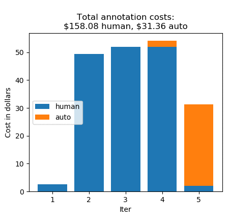
Without automatic data labeling, the annotations would have cost $0.26 * 1000, which equals $260. Instead, you paid $158.08 for 608 human labels, and $31.36 for 392 automated labels, for a total of $189.44. This is a cost saving of 27%. (For pricing details, see the Amazon SageMaker Ground Truth pricing page.)
Compare human-annotated and automated labels
Automated labels are cheap, but how do they compare to human-annotated labels? The following mIoU graph shows how well the automated labels mirror the original annotations.
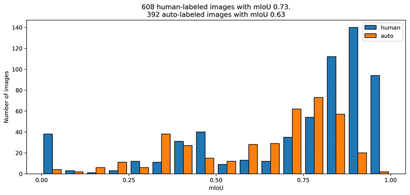
The human labelers performed slightly better on average. The automatically labeled images have an average mIoU of just above 0.6. This is the label quality that you asked the automatic labeler for. Let’s look at the top 5 images with the highest confidence scores annotated by humans and automatically labeled:


Conclusion
With automated data labeling, Ground Truth decreased bounding box annotation cost by 27%. This number will vary from dataset to dataset. It might decrease for image classification (where human annotation is cheap) and increase for semantic segmentation (where human annotation is expensive).
Feel free to experiment with or modify the Jupyter notebook. Check out our demos for other image annotation tasks – they can be accessed on any SageMaker instance, in the same way as the Jupyter notebook we just looked at!
About the authors
 Krzysztof Chalupka is an applied scientist in the Amazon ML Solutions Lab. He has a PhD in causal inference and computer vision from Caltech. At Amazon, he figures out ways in which computer vision and deep learning can augment human intelligence. His free time is filled with family. He also loves forests, woodworking, and books (trees in all forms).
 Tristan McKinney is an applied scientist in the Amazon ML Solutions Lab. He recently completed his PhD in theoretical physics at Caltech where he studied effective field theory and its application to high-T_c superconductors. As his father was in the US Army, he lived all over the place when growing up, including Germany and Albania. In his spare time, Tristan loves to ski and play soccer.
 Fedor Zhdanov is a Machine Learning Scientist at Amazon. He works on developing Machine Learning algorithms and tools for our internal and external customers.