Monitoring discriminative ML models using Amazon SageMaker AI with MLflow

The effectiveness and accuracy of machine learning (ML) models decreases almost as soon as the training job finishes. Changes in consumer behavior, releases of new products, upgrades in sensor technology, and a shifting economic and political landscape are all examples of uncontrollable factors that change the patterns and probabilities the model learned during training. By actively monitoring models deployed in production for changes in accuracy and baseline statistics, you can intervene before the drop in accuracy becomes problematic. Model monitoring can be combined with AI observability tools that track latency, application availability, and other metrics used to identify problems in the overall system.

This post focuses on discriminative machine learning models used for classification and regression use cases. For generative AI models, see Production-Ready Real-Time Monitoring Solution for LLMs on Amazon SageMaker AI Endpoint inference. The factors that cause a reduction in quality for discriminative ML models can be broadly split into two categories:

• Data drift refers to changes in the statistical properties of the input data. It can be as simple as an unexpected change in an upstream data source that changes a column from integer to float data type, or as complex as entirely new product lines being released. You can measure data drift by calculating baseline statistics for the training dataset and comparing these to the same statistics calculated on data gathered over time in production.
• Model drift refers to changes in the accuracy of predictions produced by the model because the probabilistic patterns learned by the model no longer fit the data coming in. This can be caused, for example, by changes in consumer behavior because of an improving economy. You can measure model drift by gathering the ground truth labels to calculate model quality metrics, and comparing these metrics to the same metrics calculated during the model training process.

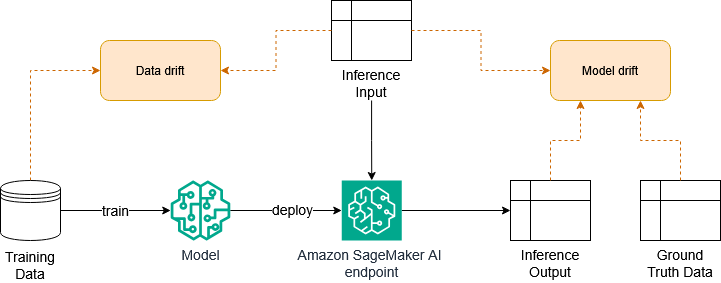
Figure 1: How data drift and model drift fit in an ML workflow

Amazon SageMaker AI is a fully managed machine learning service that helps organizations build, train, deploy, and manage both discriminative and generative ML models. Although SageMaker AI is fully managed, you might need a more customizable approach. For example, you might want to manage the entire modeling life cycle cost-effectively, monitor unique use cases that managed services do not support, or integrate your model monitoring into other UI or observability pipelines. Therefore, this post introduces a model monitoring architecture based on the open source Evidently Python library and Amazon SageMaker AI with MLflow for calculating data and model drift. The results of this model monitoring solution can be integrated into your preferred dashboard, can be used to send alerts to relevant stakeholders, or can trigger automatic model retraining pipelines.

Solution overview

This solution demonstrates how to implement model monitoring in the machine learning workflow, from model training to model deployment. Figure 2 shows the workflow for a batch inference use case, up to and including alerting in Slack and visualizing the model results in MLflow.

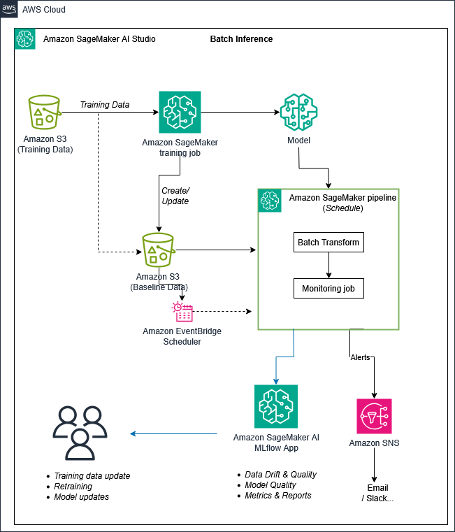
Figure 2: Model monitoring workflow for batch inference

The workflow consists of the following steps:

1. A training job to train the model on input data from an Amazon Simple Storage Service (Amazon S3) bucket. The same training job calculates model metrics, which can be stored in MLflow. The baseline dataset used to train the model is stored separately in S3 so it can be used to monitor the model in production.
2. Batch transform for inference on production workloads. The results of a batch transform job are stored in an S3 bucket.
3. The results of the batch transform job, and the original dataset and model metrics, are used in a processing job to calculate data drift and model quality metrics using open source Evidently presets. Note that Evidently calculates model metrics. It does not calculate model drift directly by comparing the metrics to the previous metrics from the training run. However, the processing job can be extended with custom code to calculate model drift. The batch transform and processing job can be wrapped in a pipeline for scheduling using Amazon EventBridge Scheduler.
4. All monitoring metrics and Evidently reports are stored in MLflow where you can track runs over time, compare results between runs, and visualize the report.
5. Optionally, if drift is detected, the pipeline can trigger an Amazon Simple Notification Service (Amazon SNS) notification to alert users by email.

You can take a similar approach for use cases where real-time endpoints are used for model deployment. Figure 3 shows the workflow for real-time endpoints. The key difference is that the endpoint must have data capture enabled, which logs the inputs and outputs of the endpoint to an S3 bucket. Instead of a processing job, this architecture uses AWS Lambda functions to deploy the monitoring code. Both architectures can use either processing jobs or Lambda, based on your preference. The AWS Lambda functions that calculate data and model drift can run on a regular schedule. You can also trigger them when data from the endpoint lands in the S3 bucket.

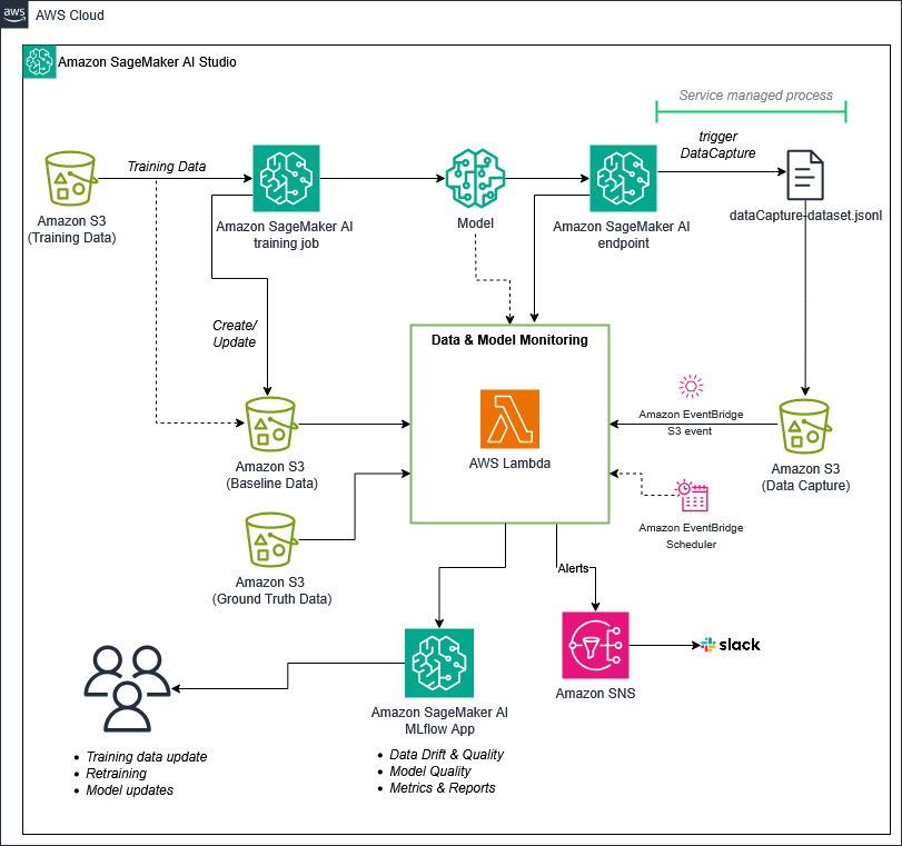
Figure 3: Model monitoring workflow for real-time endpoints

This pattern for real-time endpoints can also be used with Amazon SageMaker Hyperpod, where you can provision clusters to use for model training as well as model inference. You can enable data capture for Hyperpod at the endpoint level, at the load balancer level, or at the model pod level. Inference requests and responses are automatically written to an S3 bucket, where you can access them to perform model monitoring.

Both previous diagrams focus only on the model monitoring process. However, model monitoring is normally implemented as part of a larger MLOps workflow. Figure 4 shows how this model monitoring solution fits in an end-to-end MLOps scenario, where the processing job used to calculate drift is deployed alongside the endpoint through a CI/CD workflow. For more information on implementing MLOps with SageMaker AI, see MLOps foundation roadmap for enterprises with Amazon SageMaker AI.

Figure 4: How model monitoring integrates with an MLOps architecture

Walkthrough

This section provides a step-by-step explanation for setting up the model monitoring solution for batch transform. See the full repository for other examples, including a sample for real-time endpoints.

Prerequisites

Before following the steps in this walkthrough, you will need:

1. An Amazon SageMaker AI domain in an AWS Region where this service is available.
2. An MLflow App in SageMaker Studio.
3. A JupyterLab space within SageMaker Studio (an ml.t3.medium instance is sufficient for this solution).
4. A copy of the solution repository on JupyterLab. Clone the repository after the space has started.

To continue with the walkthrough, open the notebook predictive_ml_experimentation_data_model_monitoring_evidently.ipynb. Note that the solution uses the SageMaker Python SDK v3. If you use the DefaultMLFlowApp, the notebook code identifies the correct app automatically. Otherwise, edit the code with the name of your MLflow App.

Model training and inference

The example notebook uses the Bank Marketing dataset from the UCI Machine Learning Repository. This dataset contains information about marketing phone calls made on behalf of a Portuguese bank, with the goal of predicting if the customer will subscribe to a term deposit. It is a binary classification use case where the target variable has a value of 1 if the customer subscribed and 0 if a customer did not subscribe.

In the first half of the notebook, the data is cleaned, processed, and split into training, validation, and test sets. An XGBoost model is trained on the training and validation datasets, with logs and metrics sent to MLflow and the final model object registered in the MLflow model registry.

Two key actions in this data processing and model training section set up the model for monitoring later in production:

1. The training dataset is stored as the baseline dataset in an S3 bucket, which you use to calculate data drift.
2. The model metrics are stored in MLflow, which can be used for model drift calculations.

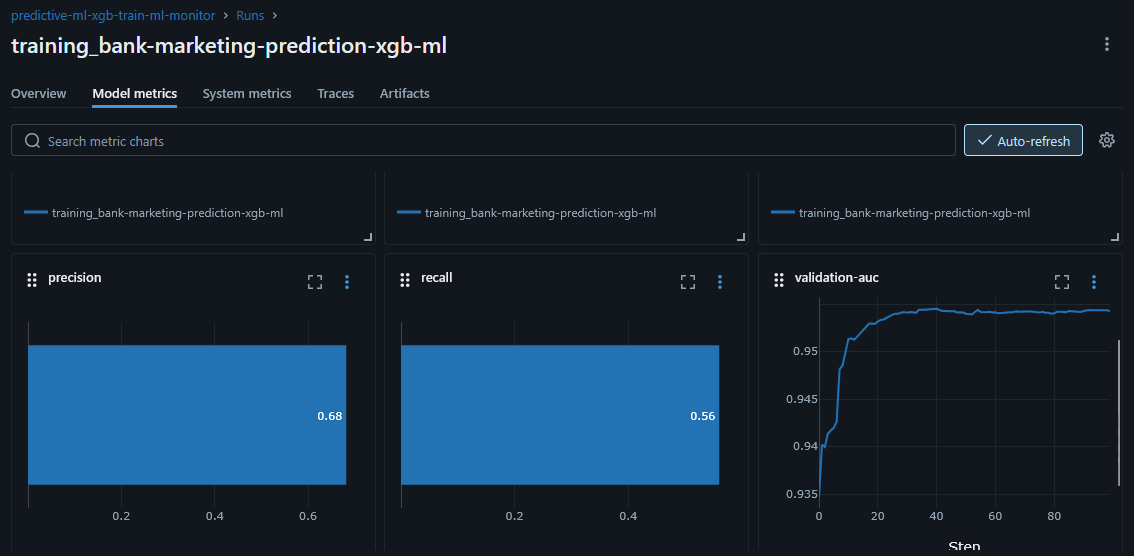
Figure 5: Model metrics (precision, recall, AUC) displayed in MLflow

Next, the notebook creates the model object from the training job output and sets up a batch transform job which runs the test features through the model for inference.

Calculating data drift and model quality

Evidently has various presets for calculating different types of data drift, all of which can be customized to suit the particular ML use case. The sample notebook uses the DataDriftPreset and DataSummaryPreset and creates a helper function to save the Evidently reports (both HTML and JSON) in MLflow and extracts specific drift values to save separately as metrics in MLflow. This enables you to compare different runs or generate alerts based on certain values.

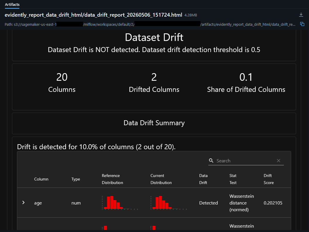
Figure 6: An Evidently data drift report as an artifact in MLflow

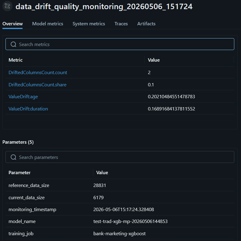
Figure 7: Data drift metrics and parameters in MLflow

Another advantage of saving each data drift calculation as a run in MLflow is that it allows us to add parameters such as the model name, the name of the training job, the size of the dataset, and other important information.

Evidently also provides presets for calculating model quality. This notebook uses the ClassificationPreset, which calculates accuracy, precision, recall, F1 score, and more based on model predictions and the ground truth dataset. Instead of the ClassificationPreset with its broad range of metrics, Evidently also supports custom reports that you can target to calculate the metrics most relevant to a particular use case. For example, because of imbalanced labels in the marketing dataset used in the sample notebook, accuracy is a less relevant metric than precision, recall, and AUC.

Similar to data monitoring, the Evidently reports for model quality are added as artifacts to MLflow, and the individual metrics can be extracted into MLflow metrics. Note that Evidently does not calculate model drift, meaning the difference between metrics from the original training job and metrics calculated from the predictions. However, you can add drift calculations in the monitoring code, and we provide an example of this in the real-time endpoint sample, where model drift, when detected, triggers an alert via Amazon SNS.

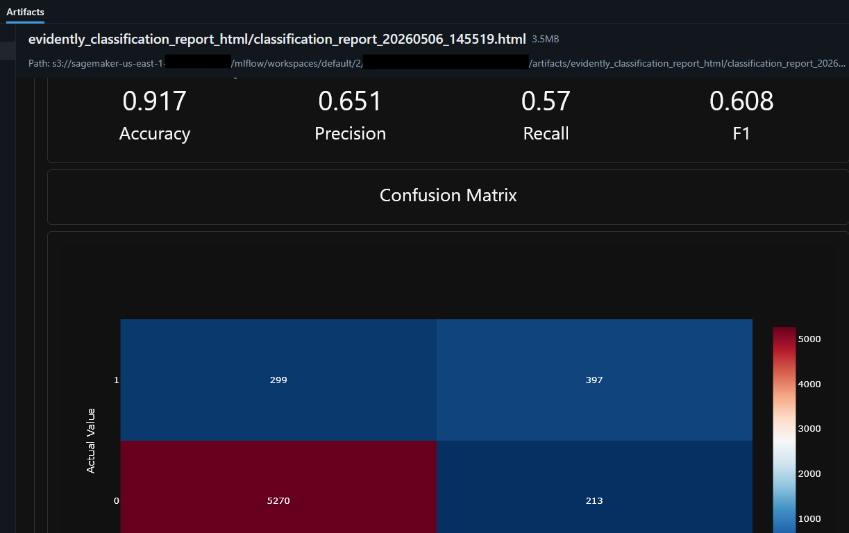
Figure 8: Model quality report artifact in MLflow

Views in MLflow can be customized and individual runs can be compared based on certain attributes. Figure 9 shows a view of multiple data drift, model quality, and comprehensive quality runs together with the original training job. You can see which training run the monitoring runs relate to, how many drifted columns were detected in the consecutive data drift runs, and how much the accuracy dropped between training and running the model quality job.

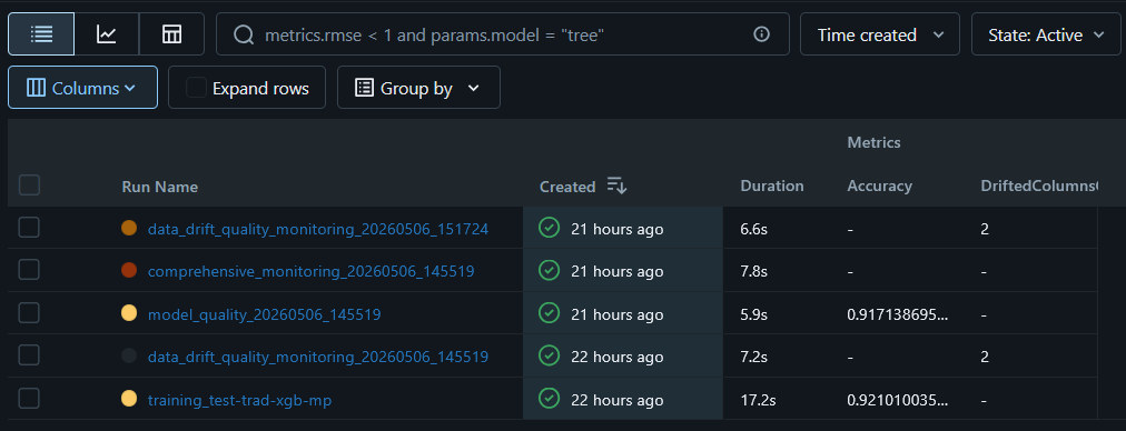
Figure 9: Multiple monitoring runs in MLflow

Furthermore, you can plot the metrics captured in MLflow over time. As shown in Figure 10, this lets you view the entire model life cycle in one place, covering model experimentation, model training, and model deployment and monitoring.

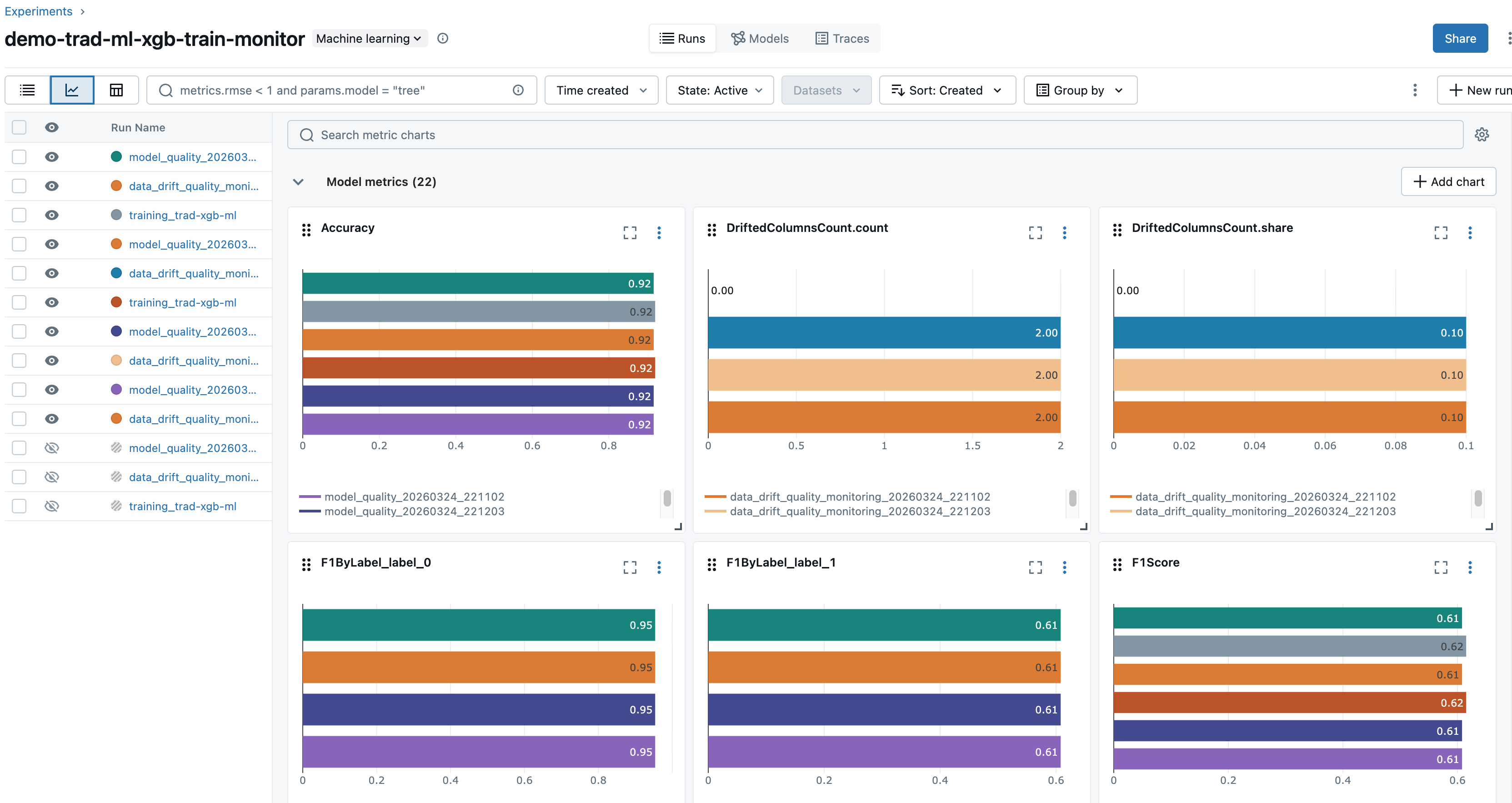
Figure 10: Model life cycle tracking metrics view in MLflow

Scaling with pipelines

Although the first notebook demonstrates in depth how to train a model, deploy it, and run monitoring with Evidently, the second notebook batch_monitoring_pipeline.ipynb shows how to scale inference and monitoring through jobs and pipelines. It creates a pipeline with two steps:

1. A Transform step that fetches the input data from S3 and runs the data through the trained XGBoost model to generate the subscription probability predictions. Predictions are stored back in S3 and passed to the next step.
2. A Processing step that uses the predictions and the baseline dataset to perform monitoring. The input dataset used to generate predictions is compared to the baseline dataset to calculate data drift, and the reports are added to MLflow.

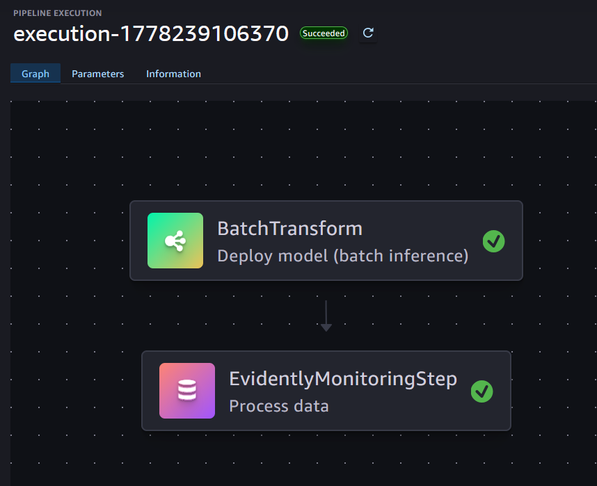
Figure 11: A pipeline with one batch transform step and one monitoring step

Finally, the notebook demonstrates how pipeline executions can be run on a regular schedule with Amazon EventBridge. For an example of how to trigger pipeline executions based on inference data becoming available in S3, see the real-time endpoint sample.

Clean up

Each notebook has a section at the end to help you clean up the resources you deployed, including any endpoints and model objects. If you wish to delete the data artifacts in S3 or the runs logged to MLflow, you need to remove them manually.

Conclusion

Implementing a data and model monitoring solution is necessary to maintain prediction accuracy and help achieve the best outcome for your machine learning use case. This post shows how you can use open source Evidently together with Amazon SageMaker AI to generate monitoring reports, organize and compare the results in MLflow, scale through pipelines, and trigger drift notifications. The AWS sample GitHub repository provides implementations for both batch predictions and real-time endpoints, with scaling done either through SageMaker AI pipelines or AWS Lambda. To learn more about MLOps on Amazon SageMaker AI, see the Amazon SageMaker AI MLOps workshop.

About the authors