Optimizing LLM inference on Amazon SageMaker AI with BentoML’s LLM- Optimizer

The rise of powerful large language models (LLMs) that can be consumed via API calls has made it remarkably straightforward to integrate artificial intelligence (AI) capabilities into applications. Yet despite this convenience, a significant number of enterprises are choosing to self-host their own models—accepting the complexity of infrastructure management, the cost of GPUs in the serving stack, and the challenge of keeping models updated. The decision to self-host often comes down to two critical factors that APIs cannot address. First, there is data sovereignty: the need to make sure that sensitive information does not leave the infrastructure, whether due to regulatory requirements, competitive concerns, or contractual obligations with customers. Second, there is model customization: the ability to fine tune models on proprietary data sets for industry-specific terminology and workflows or create specialized capabilities that general-purpose APIs cannot offer.

Amazon SageMaker AI addresses the infrastructure complexity of self-hosting by abstracting away the operational burden. Through managed endpoints, SageMaker AI handles the provisioning, scaling, and monitoring of GPU resources, allowing teams to focus on model performance rather than infrastructure management. The system provides inference-optimized containers with popular frameworks like vLLM pre-configured for maximum throughput and minimal latency. For instance, the Large Model Inference (LMI) v16 container image uses vLLM v0.10.2, which uses the V1 engine and comes with support for new model architectures and new hardware, such as the Blackwell/SM100 generation. This managed approach transforms what typically requires dedicated machine learning operations (MLOps) expertise into a deployment process that takes just a few lines of code.

Achieving optimal performance with these managed containers still requires careful configuration. Parameters like tensor parallelism degree, batch size, maximum sequence length, and concurrency limits can dramatically impact both latency and throughput—and finding the right balance for your specific workload and cost constraints is an iterative process that can be time-consuming.

BentoML’s LLM-Optimizer addresses this challenge by enabling systematic benchmarking across different parameter configurations, replacing manual trial-and-error with an automated search process. The tool allows you to define constraints such as specific latency targets or throughput requirements, making it straightforward to identify configurations that meet your service level objectives. You can use LLM-Optimizer to find optimal serving parameters for vLLM locally or in your development environment, apply those same configurations directly to the SageMaker AI endpoint for a seamless transition to production. This post illustrates this process by finding an optimal deployment for a Qwen-3-4B model on an Amazon SageMaker AI endpoint.

This post is written for practicing ML engineers, solutions architects, and system builders who already deploy models on Amazon SageMaker or similar infrastructure. We assume familiarity with GPU instances, endpoints, and model serving, and focus on practical performance optimization. The explanations of inference metrics are included not as a beginner tutorial, but to build shared intuition. For specific parameters like batch size & tensor parallelism, and how they directly impact cost and latency in production.

Solution overview

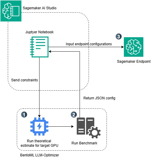
The step-by-step breakdown is as follows:

1. Define constraints in Jupyter Notebook: The process begins inside SageMaker AI Studio, where users open a Jupyter Notebook to define the deployment goals and constraints of the use case. These constraints can include target latency, desired throughput, and output tokens.
2. Run theoretical and empirical benchmarks with the BentoML LLM-Optimizer: The LLM-Optimizer first runs a theoretical GPU performance estimate to identify feasible configurations for the selected hardware (in this example, an ml.g6.12xlarge). It executes benchmark tests using the vLLM serving engine across multiple parameter combinations such as tensor parallelism, batch size, and sequence length to empirically measure latency and throughput. Based on these benchmarks, the optimizer automatically determines the most efficient serving configuration that satisfies the provided constraints.
3. Generate and deploy optimized configuration in a SageMaker endpoint: Once the benchmarking is complete, the optimizer returns a JSON configuration file containing the optimal parameter values. This JSON is passed from the Jupyter Notebook to the SageMaker Endpoint configuration, which deploys the LLM (in this example, the Qwen/Qwen3-4B model using the vLLM-based LMI container) in a managed HTTP endpoint using the optimal runtime parameters.

The following figure is an overview of the workflow conducted throughout the post.

Before jumping into the theoretical underpinnings of inference optimization, it’s worth grounding why these concepts matter in the context of real-world deployments. When teams move from API-based models to self-hosted endpoints, they inherit the responsibility for tuning performance parameters that directly affect cost and user experience. Understanding how latency and throughput interact through the lens of GPU architecture and arithmetic intensity enables engineers to make these trade-offs deliberately rather than by trial and error.

Brief overview of LLM performance

Before diving into the practical application of this workflow, we cover key concepts that build intuition for why inference optimization is critical for LLM-powered applications. The following primer isn’t academic; it is to provide the mental model needed to interpret LLM-Optimizer’s outputs and understand why certain configurations yield better results.

Key performance metrics

Throughput (requests/second): How many requests your system completes per second. Higher throughput means serving more users simultaneously.

Latency (seconds): The total time from when a request arrives until the complete response is returned. Lower latency means faster user experience.

Arithmetic intensity: The ratio of computation performed to data moved. This determines whether your workload is:

Memory-bound: Limited by how fast you can move data (low arithmetic intensity)

Compute-bound: Limited by raw GPU processing power (high arithmetic intensity)

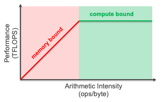
The roofline model

The roofline model visualizes performance by plotting throughput against arithmetic intensity. For deeper content on the roofline model, visit the AWS Neuron Batching documentation. The model reveals whether your application is bottlenecked by memory bandwidth or computational capacity. For LLM inference, this model helps identify if you’re limited by:

• Memory bandwidth: Data transfer between GPU memory and compute units (typical for small batch sizes)
• Compute capacity: Raw floating-point operations (FLOPS) available on the GPU (typical for large batch sizes)

The throughput-latency trade-off

In practice, optimizing LLM inference follows a fundamental trade-off: as you increase throughput, latency rises. This happens because:

• Larger batch sizes → More requests processed together → Higher throughput
• More concurrent requests → Longer queue wait times → Higher latency
• Tensor parallelism → Distributes model across GPUs → Affects both metrics differently

The challenge lies in finding the optimal configuration across multiple interdependent parameters:

• Tensor parallelism degree (how many GPUs to use)
• Batch size (maximum number of tokens processed together)
• Concurrency limits (maximum number of simultaneous requests)
• KV cache allocation (memory for attention states)

Each parameter affects throughput and latency differently while respecting hardware constraints like GPU memory and compute bandwidth. This multi-dimensional optimization problem is precisely why LLM-Optimizer is valuable—it systematically explores the configuration space rather than relying on manual trial-and-error.

For an overview on LLM Inference as a whole, BentoML has provided valuable resources in their LLM Inference Handbook.

Practical application: Finding an optimal deployment of Qwen3-4B on Amazon SageMaker AI

In the following sections, we walk through a hands-on example of identifying and applying optimal serving configurations for LLM deployment. Specifically, we:

1. Deploy the Qwen/Qwen3-4B model using vLLM on an ml.g6.12xlarge instance (4x NVIDIA L4 GPUs, 24GB VRAM each).
2. Define realistic workload constraints:
   • Target: 10 requests per second (RPS)
   • Input length: 1,024 tokens
   • Output length: 512 tokens
3. Explore multiple serving parameter combinations:
   • Tensor parallelism degree (1, 2, or 4 GPUs)
   • Max batched tokens (4K, 8K, 16K)
   • Concurrency levels (32, 64, 128)
4. Analyze results using:
   • Theoretical GPU memory calculations
   • Benchmarking data
   • Throughput vs. latency trade-offs

By the end, you’ll see how theoretical analysis, empirical benchmarking, and managed endpoint deployment come together to deliver a production-ready LLM setup that balances latency, throughput, and cost.

Prerequisites

The following are the prerequisites needed to run through this example:

• Access to SageMaker Studio. This makes deployment & inference straightforward, or an interactive development environment (IDE) such as PyCharm or Visual Studio Code.
• To benchmark and deploy the model, check that the recommended instance types are accessible, based on the model size. To verify the necessary service quotas, complete the following steps:
  • On the Service Quotas console, under AWS Services, select Amazon SageMaker.
  • Verify sufficient quota for the required instance type for “endpoint deployment” (in the correct region).
  • If needed, request a quota increase/contact AWS for support.

The following code details how to install the necessary packages:

pip install vllm
pip install git+https://github.com/bentoml/llm-optimizer.git 

Run the LLM-Optimizer

To get started, example constraints must be defined based on the targeted workflow.

Example constraints:

• Input tokens: 1024
• Output tokens: 512
• E2E Latency: <=  60 seconds
• Throughput: >= 5 RPS

Run the estimate

The first step with llm-optimizer is to run an estimation. Running an estimate analyzes the Qwen/Qwen3-4b model on 4x L4 GPUs and estimate the performance for an input length of 1024 tokens, and an output of 512 tokens. Once run, the theoretical bests for latency and throughput are calculated mathematically and returned. The roofline analysis returned identifies the workloads bottlenecks, and a number of server and client arguments are returned, for use in the following step, running the actual benchmark.

Under the hood, LLM-Optimizer performs roofline analysis to estimate LLM serving performance. It starts by fetching the model architecture from HuggingFace to extract parameters like hidden dimensions, number of layers, attention heads, and total parameters. Using these architectural details, it calculates the theoretical FLOPs required for both prefill (processing input tokens) and decode (generating output tokens) phases, accounting for attention operations, MLP layers, and KV cache access patterns. It compares the arithmetic intensity (FLOPs per byte moved) of each phase against the GPU’s hardware characteristics—specifically the ratio of compute capacity (TFLOPs) to memory bandwidth (TB/s)—to determine whether prefill and decode are memory-bound or compute-bound. From this analysis, the tool estimates TTFT (time-to-first-token), ITL (inter-token latency), and end-to-end latency at various concurrency levels. It also calculates three theoretical concurrency limits: KV cache memory capacity, prefill compute capacity, and decode throughput capacity. Finally, it generates tuning commands that sweep across different tensor parallelism configurations, batch sizes, and concurrency levels for empirical benchmarking to validate the theoretical predictions.

The following code details how to run an initial estimation based on the selected constraints:

llm-optimizer estimate \ 
--model Qwen/Qwen3-4B \ 
--input-len 1024 \ 
--output-len 512 \ 
--gpu L40 \ 
--num-gpus 4

Expected output:

Auto-detected 4 GPU(s)
💡 Inferred precision from model config: bf16

=== Configuration ===
Model: Qwen/Qwen3-4B
GPU: 4x L40
Precision: bf16
Input/Output: 1024/512 tokens
Target: throughput

Fetching model configuration...
Model: 3668377600.0B parameters, 36 layers

=== Performance Analysis ===
Best Latency (concurrency=1):
  TTFT: 16.8 ms
  ITL: 1.4 ms
  E2E: 0.72 s

Best Throughput (concurrency=1024):
  Output: 21601.0 tokens/s
  Input: 61062.1 tokens/s
  Requests: 24.71 req/s
  Bottleneck: Memory

=== Roofline Analysis ===
Hardware Ops/Byte Ratio: 195.1 ops/byte
Prefill Arithmetic Intensity: 31846.2 ops/byte
Decode Arithmetic Intensity: 31.1 ops/byte
Prefill Phase: Compute Bound
Decode Phase: Memory Bound

=== Concurrency Analysis ===
KV Cache Memory Limit: 1258 concurrent requests
Prefill Compute Limit: 21 concurrent requests
Decode Capacity Limit: 25 concurrent requests
Theoretical Overall Limit: 21 concurrent requests
Empirical Optimal Concurrency: 16 concurrent requests

=== Tuning Commands ===

--- VLLM ---
Simple (concurrency + TP/DP):
  llm-optimizer --framework vllm --model Qwen/Qwen3-4B --gpus 4 --host 127.0.0.1 --server-args "tensor_parallel_size*data_parallel_size=[(1, 4), (2, 2), (4, 1)]" --client-args "dataset_name=random;random_input_len=1024;random_output_len=512;random_range_ratio=0.95;num_prompts=3072;max_concurrency=[512, 1024, 1536]" --output-dir tuning_results --output-json tuning_results/config_1_vllm.json
Advanced (additional parameters):
  llm-optimizer --framework vllm --model Qwen/Qwen3-4B --gpus 4 --host 127.0.0.1 --server-args "tensor_parallel_size*data_parallel_size=[(1, 4), (2, 2), (4, 1)];max_num_batched_tokens=[16384, 24576, 32768]" --client-args "dataset_name=random;random_input_len=1024;random_output_len=512;random_range_ratio=0.95;num_prompts=3072;max_concurrency=[512, 1024, 1536]" --output-dir tuning_results --output-json tuning_results/config_1_vllm.json

Run the benchmark

With the estimation outputs in hand, an informed decision can be made on what parameters to use for benchmarking based on the previously defined constraints. Under the hood, LLM-Optimizer transitions from theoretical estimation to empirical validation by launching a distributed benchmarking loop that evaluates real-world serving performance on the target hardware. For each permutation of server and client arguments, the tool automatically spins up a vLLM instance with the specified tensor parallelism, batch size, and token limits, then drives load using a synthetic or dataset-based request generator (e.g., ShareGPT). Each run captures low-level metrics—time-to-first-token (TTFT), inter-token latency (ITL), end-to-end latency, tokens per second, and GPU memory utilization—across concurrent request patterns. These measurements are aggregated into a Pareto frontier, allowing LLM-Optimizer to identify configurations that best balance latency and throughput within the user’s constraints. In essence, this step grounds the earlier theoretical roofline analysis in real performance data, producing reproducible metrics that directly inform deployment tuning.

The following code runs the benchmark, using information from the estimate:

llm-optimizer \
  --framework vllm \
  --model Qwen/Qwen3-4B \
  --server-args "tensor_parallel_size=[1,2,4];max_num_batched_tokens=[4096,8192,16384]" \
  --client-args "max_concurrency=[32,64,128];num_prompts=1000;dataset_name=sharegpt" \
  --output-json vllm_results.json

This outputs the following permutations to the vLLM engine for testing. The following are simple calculations on the different combinations of client & server arguments that the benchmark runs:

• 3 tensor_parallel_size x 3 max_num_batched_tokens settings = 9
• 3 max_concurrency x 1 num prompts = 3
• 9 * 3 = 27 different tests

Once completed, three artifacts are generated:

1. An HTML file containing a Pareto dashboard of the results: An interactive visualization that highlights the trade-offs between latency and throughput across the tested configurations.
2. A JSON file summarizing the benchmark results: This compact output aggregates the key performance metrics (e.g., latency, throughput, GPU utilization) for each test permutation and is used for programmatic analysis or downstream automation.
3. A JSONL file containing the full record of individual benchmark runs: Each line represents a single test configuration with detailed metadata, enabling fine-grained inspection, filtering, or custom plotting.

Example benchmark record output:

{"config": {"client_args": {"max_concurrency": 32, "num_prompts": 1000, "dataset_name": "sharegpt"}, "server_args": {"tensor_parallel_size": 4, "max_num_batched_tokens": 8192}, "server_cmd_args": ["--tensor-parallel-size=4", "--max-num-batched-tokens=8192"]}, "results": {"backend": "vllm", "dataset_name": "sharegpt", "max_concurrency": 32, "duration": 178.69010206999883, "completed": 1000, "total_input_tokens": 302118, "total_output_tokens": 195775, "total_output_tokens_retokenized": 195764, "request_throughput": 5.5962808707125085, "input_throughput": 1690.7371840979215, "output_throughput": 1095.6118874637414, "mean_e2e_latency_ms": 5516.473195931989, "median_e2e_latency_ms": 3601.3218250000136, "std_e2e_latency_ms": 6086.249975393793, "p95_e2e_latency_ms": 17959.23558074991, "p99_e2e_latency_ms": 23288.202798799084, "mean_ttft_ms": 134.24923809297798, "median_ttft_ms": 75.87540699933015, "std_ttft_ms": 219.7887602629944, "p95_ttft_ms": 315.9690581494033, "p99_ttft_ms": 1222.5397153301492, "mean_tpot_ms": 28.140094508604655, "median_tpot_ms": 27.28665116875758, "std_tpot_ms": 7.497764233364623, "p95_tpot_ms": 36.30593537913286, "p99_tpot_ms": 48.05242155004177, "mean_itl_ms": 27.641122410215683, "median_itl_ms": 21.38108600047417, "std_itl_ms": 28.983685761892183, "p95_itl_ms": 64.98022639971161, "p99_itl_ms": 133.48110956045272, "concurrency": 30.871733420192484, "accept_length": null}, "cmd": "vllm serve Qwen/Qwen3-4B --host 127.0.0.1 --port 8000 --tensor-parallel-size=4 --max-num-batched-tokens=8192", "constraints": [], "metadata": {"gpu_type": "NVIDIA L4", "gpu_count": 4, "model_tag": "Qwen/Qwen3-4B", "input_tokens": -1, "output_tokens": -1}}
{"config": {"client_args": {"max_concurrency": 64, "num_prompts": 1000, "dataset_name": "sharegpt"}, "server_args": {"tensor_parallel_size": 4, "max_num_batched_tokens": 8192}, "server_cmd_args": ["--tensor-parallel-size=4", "--max-num-batched-tokens=8192"]}, "results": {"backend": "vllm", "dataset_name": "sharegpt", "max_concurrency": 64, "duration": 151.1696548789987, "completed": 1000, "total_input_tokens": 302118, "total_output_tokens": 195775, "total_output_tokens_retokenized": 195768, "request_throughput": 6.615084229704922, "input_throughput": 1998.5360173099916, "output_throughput": 1295.068115070481, "mean_e2e_latency_ms": 8939.159275709007, "median_e2e_latency_ms": 6008.622306500911, "std_e2e_latency_ms": 9605.635172303826, "p95_e2e_latency_ms": 27139.969452801306, "p99_e2e_latency_ms": 37183.75254391998, "mean_ttft_ms": 251.3472756509782, "median_ttft_ms": 116.74506849976751, "std_ttft_ms": 491.6096066277092, "p95_ttft_ms": 1224.981592999029, "p99_ttft_ms": 2902.0978502906837, "mean_tpot_ms": 48.65581712437634, "median_tpot_ms": 45.59879392866151, "std_tpot_ms": 31.47685312628492, "p95_tpot_ms": 65.96288688333136, "p99_tpot_ms": 130.59083745436504, "mean_itl_ms": 44.61668980280019, "median_itl_ms": 33.35350599991216, "std_itl_ms": 44.581804322583615, "p95_itl_ms": 111.47860099845275, "p99_itl_ms": 222.5829249997332, "concurrency": 59.133291551563126, "accept_length": null}, "cmd": "vllm serve Qwen/Qwen3-4B --host 127.0.0.1 --port 8000 --tensor-parallel-size=4 --max-num-batched-tokens=8192", "constraints": [], "metadata": {"gpu_type": "NVIDIA L4", "gpu_count": 4, "model_tag": "Qwen/Qwen3-4B", "input_tokens": -1, "output_tokens": -1}}
{"config": {"client_args": {"max_concurrency": 128, "num_prompts": 1000, "dataset_name": "sharegpt"}, "server_args": {"tensor_parallel_size": 4, "max_num_batched_tokens": 8192}, "server_cmd_args": ["--tensor-parallel-size=4", "--max-num-batched-tokens=8192"]}, "results": {"backend": "vllm", "dataset_name": "sharegpt", "max_concurrency": 128, "duration": 133.0894289429998, "completed": 1000, "total_input_tokens": 302118, "total_output_tokens": 195775, "total_output_tokens_retokenized": 195771, "request_throughput": 7.513744765020255, "input_throughput": 2270.0375409183894, "output_throughput": 1471.0033813718405, "mean_e2e_latency_ms": 14910.240386960006, "median_e2e_latency_ms": 10384.713371499856, "std_e2e_latency_ms": 15223.620712896502, "p95_e2e_latency_ms": 43486.963950149395, "p99_e2e_latency_ms": 61421.81745829036, "mean_ttft_ms": 663.0696945789732, "median_ttft_ms": 189.89979050093098, "std_ttft_ms": 1407.5295299267668, "p95_ttft_ms": 4652.777336598592, "p99_ttft_ms": 7000.883197711337, "mean_tpot_ms": 91.83800469031593, "median_tpot_ms": 77.46479336456856, "std_tpot_ms": 94.19538916493616, "p95_tpot_ms": 125.3206487750731, "p99_tpot_ms": 500.0748501195875, "mean_itl_ms": 73.16857466775902, "median_itl_ms": 49.85373300041829, "std_itl_ms": 72.57371615955182, "p95_itl_ms": 172.3669967985188, "p99_itl_ms": 328.1056552407972, "concurrency": 112.03174065271433, "accept_length": null}, "cmd": "vllm serve Qwen/Qwen3-4B --host 127.0.0.1 --port 8000 --tensor-parallel-size=4 --max-num-batched-tokens=8192", "constraints": [], "metadata": {"gpu_type": "NVIDIA L4", "gpu_count": 4, "model_tag": "Qwen/Qwen3-4B", "input_tokens": -1, "output_tokens": -1}}

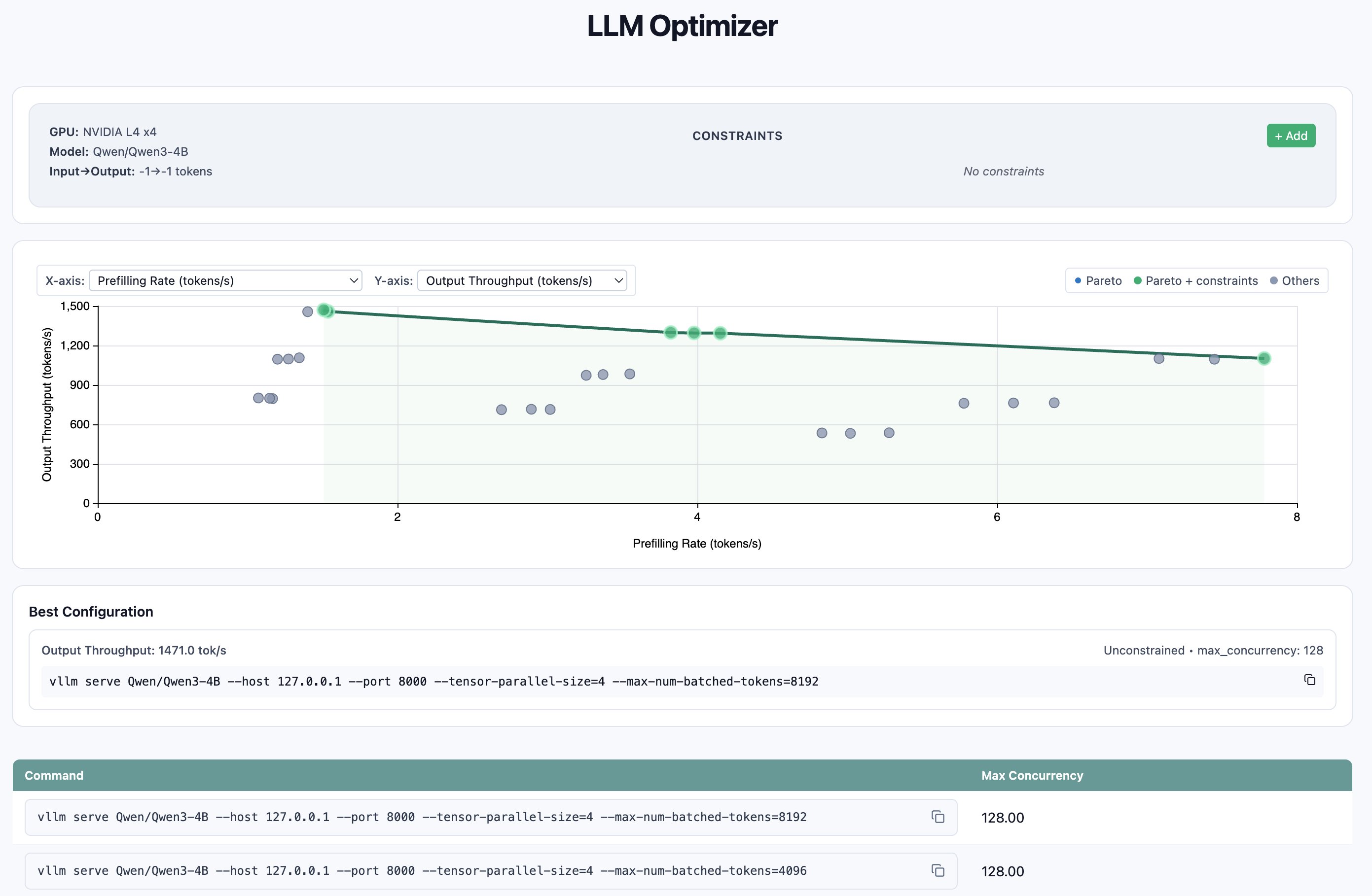
Unpacking the benchmark results, we can use the metrics p99 e2e latency and request throughput at various levels of concurrency to make an informed decision. The benchmark results revealed that tensor parallelism of 4 across the available GPUs consistently outperformed lower parallelism settings, with the optimal configuration being tensor_parallel_size=4, max_num_batched_tokens=8192, and max_concurrency=128, achieving 7.51 requests/second and 2,270 input tokens/second—a 2.7x throughput improvement over the naive single-GPU baseline (2.74 req/s).While this configuration delivered peak throughput, it came with elevated p99 end-to-end latency of 61.4 seconds under heavy load; for latency-sensitive workloads, the sweet spot was tensor_parallel_size=4 with max_num_batched_tokens=4096 at moderate concurrency (32), which maintained sub-24-second p99 latency while still delivering 5.63 req/s—more than double the baseline throughput. The data demonstrates that moving from a naive single-GPU setup to optimized 4-way tensor parallelism with tuned batch sizes can unlock substantial performance gains, with the specific configuration choice depending on whether the deployment prioritizes maximum throughput or latency assurances.

To visualize the results, LLM-Optimizer provides a convenient function to view the outputs plotted in a Pareto dashboard. The Pareto dashboard can be displayed with the following line of code:

llm-optimizer visualize --data-file vllm_results.json --port 8080 --serve

With the correct artifacts now in hand, the model with the correct configurations can be deployed.

Deploying to Amazon SageMaker AI

With the optimal serving parameters identified through LLM-Optimizer, the final step is to deploy the tuned model into production. Amazon SageMaker AI provides an ideal environment for this transition, abstracting away the infrastructure complexity of distributed GPU hosting while preserving fine-grained control over inference parameters. By using LMI containers, developers can deploy open-source frameworks like vLLM at scale, without managing CUDA dependencies, GPU scheduling, or load balancing manually.

SageMaker AI LMI containers are high-performance Docker images specifically designed for LLM inference. These containers integrate natively with frameworks such as vLLM and TensorRT, and offer built-in support for multi-GPU tensor parallelism, continuous batching, streaming token generation, and other optimizations critical to low-latency serving. The LMI v16 container used in this example includes vLLM v0.10.2 and the V1 engine, supporting new model architectures and improving both latency and throughput compared to previous versions.

Now that the best quantitative values for inference serving have been determined, those configurations can be passed directly to the container as environment variables. (please refer here for in-depth guidance):

env = {
    "HF_MODEL_ID": "Qwen/Qwen3-4B",
    "OPTION_ASYNC_MODE": "true",
    "OPTION_ROLLING_BATCH": "disable",
    "OPTION_ENTRYPOINT": "djl_python.lmi_vllm.vllm_async_service",
    "OPTION_MAX_ROLLING_BATCH_PREFILL_TOKENS": "8192",
    "OPTION_TENSOR_PARALLEL_DEGREE": "4",
}

When these environment variables are applied, SageMaker automatically injects them into the container’s runtime configuration layer, which initializes the vLLM engine with the desired arguments. During startup, the container downloads the model weights from Hugging Face, configures the GPU topology for tensor parallel execution across the available devices (in this case, on the ml.g6.12xlarge instance), and registers the model with the SageMaker Endpoint Runtime. This makes sure that the model runs with the same optimized settings validated by LLM-Optimizer, bridging the gap between experimentation and production deployment.

The following code demonstrates how to package and deploy the model for real-time inference on SageMaker AI:

image_uri = f"763104351884.dkr.ecr.{region}.amazonaws.com/djl-inference:0.34.0-lmi16.0.0-cu128"
model_name = name_from_base("qwen3-4b-stateful")

create_model = sm_client.create_model(
ModelName = model_name,
ExecutionRoleArn = role,
PrimaryContainer = {
"Image": image_uri,
"Environment": env,
},
)
model_arn = create_model["ModelArn"]

Once the model construct is created, you can create and activate the endpoint:

create_endpoint = sm_client.create_endpoint(
    EndpointName=endpoint_name, EndpointConfigName=endpoint_config_name
)

After deployment, the endpoint is ready to handle live traffic and can be invoked directly for inference:

request = {
    "messages": [
            {"role": "user", "content": "What is Amazon SageMaker?"}
            ],
            "max_tokens": 50,
            "temperature": 0.75,
            "stop": None
}

response_model = smr_client.invoke_endpoint(
    EndpointName=endpoint_name,
    Body=json.dumps(request),
    ContentType="application/json",
)
response = response_model["Body"].read()
response = “Amazon SageMaker is AWS's fully managed machine learning service that enables developers and data scientists to build, train, and deploy machine learning models at scale.”  

These code snippets demonstrate the deployment flow conceptually. For a complete end-to-end sample on deploying an LMI container for real time inference on SageMaker AI, refer to this example.

Conclusion

The journey from model selection to production deployment no longer needs to rely on trial and error. By combining BentoML’s LLM-Optimizer with Amazon SageMaker AI, organizations can now move from hypothesis to deployment through a data-driven, automated optimization loop. This workflow replaces manual parameter tuning with a repeatable process that quantifies performance trade-offs, aligns with business-level latency and throughput objectives, and deploys the best configuration directly into a managed inference environment. This workflow addresses a critical challenge in production LLM deployment: without systematic optimization, teams face an expensive guessing game between over-provisioning GPU resources and risking degraded user experience. As demonstrated in this walkthrough, the performance differences are substantial—misconfigured setups can require 2-4x more GPUs while delivering 2-3x higher latency. What could traditionally take an engineer days or weeks of manual trial-and-error testing becomes a few hours of automated benchmarking. By combining LLM-Optimizer’s intelligent configuration search with SageMaker AI’s managed infrastructure, teams can make data-driven deployment decisions that directly impact both cloud costs and user satisfaction, focusing their efforts on building differentiated AI experiences rather than tuning inference parameters.

The combination of automated benchmarking and managed large-model deployment represents a significant step forward in making enterprise AI both accessible and economically efficient. By leveraging LLM-Optimizer for intelligent configuration search and SageMaker AI for scalable, fault-tolerant hosting, teams can focus on building differentiated AI experiences rather than managing infrastructure or tuning inference stacks manually. Ultimately, the best LLM configuration isn’t just the one that runs fastest—it’s the one that meets specific latency, throughput, and cost goals in production. With BentoML’s LLM-Optimizer and Amazon SageMaker AI, that balance can be discovered systematically, reproduced consistently, and deployed confidently.

Additional resources

• LMI Container overview
• LLM-Optimizer blog
• LLM-Optimizer GitHub repository

About the authors

Josh Longenecker is a Generative AI/ML Specialist Solutions Architect at AWS, partnering with customers to architect and deploy cutting-edge AI/ML solutions. He’s part of the Neuron Data Science Expert TFC and passionate about pushing boundaries in the rapidly evolving AI landscape. Outside of work, you’ll find him at the gym, outdoors, or enjoying time with his family.

Mohammad Tahsin is a Generative AI/ML Specialist Solutions Architect at AWS, where he works with customers to design, optimize, and deploy modern AI/ML solutions. He’s passionate about continuous learning and staying on the frontier of new capabilities in the field. In his free time, he enjoys gaming, digital art, and cooking.