Artificial Intelligence
SageMaker Inference now supports Multi-Instance GPU to maximize GPU utilization for model endpoints
When you deploy a model to a GPU endpoint, the smallest unit of GPU you can request is one whole accelerator.
This constraint can cost you twice. First, you can’t host more models on an instance than it has accelerators. An ml.p4d.24xlarge has eight A100s, so it holds eight models, whether each one needs 40 GB or 14 GB. Second, and less obvious, it makes every deployment come down to a choice of which full GPU to deploy to. As your concurrency and prompt lengths grow, a full GPU on an older instance stops being enough, but a full GPU on a newer one is more than your model can use. You end up either under-served or paying for capability you never reach.
Today, Amazon SageMaker Inference supports GPU partitioning, which uses NVIDIA Multi-Instance GPU (MIG) to divide a physical GPU into independent partitions. Each partition receives a fixed share of the GPU’s compute units and a dedicated block of its memory, with isolation enforced in hardware. That changes both constraints: you can place a different model in each partition, and you can choose a fraction of a newer accelerator instead of a whole one of either generation.
This post covers both. The first part is the direct benefit: deploy more models than you have GPUs, with isolation between them. The second is the one customers ask about when the question turns to cost: how the granularity of partitioning helps you pick the right-sized unit, and what we measured when we did.
One thing to know before you read further: GPU partitioning works on endpoints that use inference components, the construct you use to deploy several models to one endpoint and set the compute each model gets. Partitioning builds directly on it. A partition is a resource a component asks for, in the same place it already asks for CPU and memory. If you haven’t used inference components, this post introduces them. Single-model endpoints, serverless endpoints, and heterogeneous instance pools cannot be partitioned.
What customers do today, and why each option falls short
If you have more models than accelerators, you have had three choices.
Run fewer, larger endpoints and batch harder – This raises utilization, but only when the models are interchangeable. A portfolio of fine-tuned variants or per-tenant models is not.
Use multi-model endpoints – These load and unload models from a shared GPU on demand, which fits sparse, bursty traffic. But models share the device without isolation, so a heavy request for one model affects the others. A model that isn’t loaded also pays a load penalty on first use.
Move to self-managed Kubernetes – This is where customers who need real GPU partitioning have gone. MIG works there, but you take on driver versioning, partition configuration, a device plugin, scheduling, and keeping it all consistent across a fleet. That’s a lot of work for a hardware capability your instances already have.
Why MIG
NVIDIA Multi-Instance GPU (MIG) splits one GPU into as many as seven instances, depending on the GPU. Each instance has its own compute, cache, memory and memory bandwidth. Because the split is in hardware rather than software, you get guarantees that other sharing methods can’t give:
- Predictable latency – Each partition has dedicated memory bandwidth, so one model’s traffic spike doesn’t show up in another model’s p99.
- Fault isolation – A crash or memory error stays inside its partition instead of taking down every model on the GPU.
- Right-sized capacity – Small and mid-sized models get a slice that fits them instead of a whole GPU. You can mix slice sizes on one device.
- No cold starts – Every model keeps its own partition and stays loaded, with no load penalty and no eviction.
- Tenant isolation – Memory protection between partitions is enforced in hardware, which makes security and compliance reviews simpler.
- Reliable planning and chargeback – A partition performs the same way regardless of its neighbors, so load tests predict production. GPU cost also maps cleanly to a model, team or tenant.
Partitioning has boundaries worth knowing up front. The maximum number of partitions depends on the accelerator and never exceeds seven. MIG itself only allows a layout to change while its partitions are idle, and on SageMaker AI that means choosing a layout when you create the endpoint. A model that needs more than one GPU still needs whole devices. Within those boundaries, you get the isolation of separate GPUs without dedicating one to each model.
Partitioning without the platform work
Until now, getting MIG meant running the Kubernetes stack yourself. GPU partitioning on Amazon SageMaker AI removes that step: you pick a partition profile for your model, and SageMaker AI handles GPU configuration, placement and scaling. You get hardware-isolated GPU sharing on a managed endpoint, without having to run the platform underneath it.
Salesforce has been part of this work from the start, helping define the requirements and validating the initial implementation.
“NVIDIA MIG partitions a single GPU into multiple isolated instances, each with dedicated compute and memory resources. Salesforce sees this as an important capability because many inference workloads do not require an entire GPU. MIG would allow us to consolidate workloads safely, significantly improve GPU utilization, reduce inference costs, and maintain predictable performance and strong isolation.
This capability would help us scale AI Inference more efficiently across different use cases. Salesforce has helped define requirements, validated the initial solution. We are now preparing to validate the solution with representative production workload and demonstrate strong customer demand with AWS. We believe MIG support would deliver meaningful technical and business value for enterprise customers.”
— Richard Chang, Software Engineering Architect, Salesforce
How it works
GPU partitioning adds two optional fields to API calls you already make. There are no new API operations, no new resource types, and no new AWS Identity and Access Management (IAM) actions, and an endpoint that omits both fields behaves exactly as it does today.
AcceleratorPartitionLayouts goes on a production variant in CreateEndpointConfig and declares how each accelerator is divided:
An A100 has seven compute slices to divide. The preceding layout uses all seven, so each of the eight A100s on the p4d instance carries three partitions and the endpoint provides 24, eight of each type.
The carve applies uniformly. One layout entry describes how one accelerator is divided, and every accelerator on every instance in the variant is divided the same way. The list isn’t positional, so an entry doesn’t map to a specific GPU.
AcceleratorPartitionType goes on an inference component and selects which partition the model runs on:
Each component copy occupies one partition of the requested type. With eight partitions of each type on the instance, raising CopyCount places additional copies on free partitions. This is useful for a small model serving high concurrency, where a single process leaves the GPU waiting on requests.
NumberOfAcceleratorDevicesRequired is always 1 here. With a partition type set it means one partition rather than one accelerator. NumberOfCpuCoresRequired and MinMemoryRequiredInMb still describe host CPU and host memory, because GPU memory comes from the partition type.
Invocation doesn’t change. InvokeEndpoint addresses a model by inference component name, and the partition it occupies never appears in the request.
Partitioning happens while the endpoint is provisioned. When it reaches InService every accelerator is carved and the partitions are empty, which is a valid state as components land on them afterward. In our testing, carving accelerators added roughly 17 seconds to provisioning. The rest of the time is the usual instance launch and container pull.
Partition profiles by GPU
The profiles available to you are a property of the GPU, so start by finding out which GPU your instance type carries and look it up in NVIDIA’s supported MIG profiles, which is the authority on the full profile set and the combinations valid on one device.
| Instance family | Accelerator | GPU memory | Granularity (compute / memory) | Available partition profiles | Max partitions per GPU |
| P4d | NVIDIA A100 | 40 GB | 7 / 8 | mig-1g.5gb, mig-1g.10gb (see driver note), mig-2g.10gb, mig-3g.20gb, mig-4g.20gb, mig-7g.40gb | 7 |
| P5 | NVIDIA H100 | 80 GB | 7 / 8 | mig-1g.10gb, mig-1g.20gb, mig-2g.20gb, mig-3g.40gb, mig-4g.40gb, mig-7g.80gb | 7 |
| G7 | NVIDIA RTX PRO 4500 Blackwell | 32 GB | 2 / 2 | mig-1g.16gb, mig-2g.32gb | 2 |
| G7e | NVIDIA RTX PRO 6000 Blackwell Server Edition | 96 GB | 4 / 4 | mig-1g.24gb, mig-2g.48gb, mig-4g.96gb | 4 |
Read the profile name as compute units followed by GPU memory: mig-3g.40gb takes three compute units and 40 GB. The granularity column is what limits a layout. An A100 and an H100 divide into sevenths on compute and eighths on memory, while G7 divides into halves and G7e into quarters. Profile names differ between GPUs even where the slice counts match, so don’t carry a layout from one instance family to another without checking it against this table.
Within those limits you have real choice. On a P4d or P5 you can carve seven of the smallest profile, or two 3g partitions, or the 4g plus 2g plus 1g layout used in the earlier example, or take the whole device as one. On a G7e you can take four of the smallest, or two 1g beside a 2g, or two 2g, or one whole device. On a G7, either two partitions or one.
The 3g profile is the one to know, because its two dimensions don’t match: it takes three of the seven compute units but four of the eight memory units. Two of them fill the GPU and nothing else will fit beside them.
The high-level rule: Every profile in your layout must be one your GPU offers, and the compute and memory units your profiles add up to must not exceed what one device provides. Both are checked when you create the endpoint configuration, and either one failing is a rejection rather than a fallback to a whole accelerator.
Driver note for P4d: mig-1g.10gb requires an R525 or newer NVIDIA driver, and the default P4d image ships 470.256.02. Request it on the default image and the carve fails without an error naming the profile. Set InferenceAmiVersion to al2023-ami-sagemaker-inference-gpu-4-1 on the production variant to get an image on the 580 driver line, which offers it.
Choosing a layout for your workload
Choosing well is a separate question from choosing a layout that is merely accepted. A partition hands you compute and memory in fixed proportions, and the two do different jobs during inference.
Compute units are what you need for prefill. Prefill reads the prompt and builds its representation. This is the compute-heavy phase, and it scales with the streaming multiprocessors, and so the TFLOPs, your partition holds. The longer your inputs and the more prompts arriving at once, the more it governs how quickly you return a first token.
Memory units are what you need for decode and for capacity. Generating tokens re-reads the model weights on every step, so decode is bounded by memory bandwidth rather than by math, and memory also caps how much KV cache you can hold. That cap in turn sets the context length you can serve and how many sequences you can serve concurrently.
Almost no real workload exercises only one of these, so the goal isn’t to pick a dimension but to choose a combination that supports your use case. Choose a profile whose proportions cover your heaviest phase while leaving the other adequately served. On the compute side, what matters is how long your prompts are and how many arrive at once. On the memory side, it’s your output length, your context window, and your concurrency.
Memory is the easier of the two to underestimate, because a partition has to hold three things and not just the model: the weights, which for an 8B model at FP16 are about 16 GB. The KV cache, sized for the context length and the number of concurrent sequences you intend to allow, which is the term people leave out and the one that grows with traffic. And 1–2 GB of runtime overhead for the CUDA context and the serving process. Add those up before choosing a profile, because a partition sized to the weights alone will load the model and then fail under load, or quietly serve a much shorter context than you configured. For a concrete reference point, that same 8B model at FP16 comfortably serves an 8,000-token context on a 40 GB partition.
Where MIG adds the most value
A portfolio of small and mid-size models – The direct case. Fine-tuned variants, embedding models, rerankers, and classifiers that each leave most of an accelerator unused now share one.
Multi-tenant model serving – When you host a model per customer, MIG gives you a hardware boundary between them: a process in one partition can’t read another partition’s memory or take its throughput. Scope the claim accurately, though. Models on the same instance still share host CPU, system memory, storage, networking, and endpoint routing, so partitioning is an isolation mechanism for the GPU and not a complete tenancy boundary.
Multi-stage pipelines on one instance – A transcription model, a diarization model, and a language model, or an embedder, a reranker, and a generator. Each stage is a separately addressable component on its own partition, and a network hop between stages disappears.
A small model in the request path – A safety classifier or guardrail model that has to run on every request but cannot justify an accelerator, with predictable latency because it isn’t time-slicing against the main model.
Challengers and canaries – Run a candidate model on a small partition beside the model serving production traffic instead of standing up a second endpoint.
Performance: A slice of a newer GPU against a whole older one
In addition to bin-packing, the other benefit you get is granularity on high-end GPUs: more GPU options to deploy a model onto, and the choice of which one is yours. Every supported accelerator becomes several sizes rather than one, so the practical way to think about it is that each profile is a GPU option in its own right, sitting alongside the whole accelerators you already choose between. That matters most when you are considering a larger or newer instance type, because moving up stops being all-or-nothing: you can take as much or as little of that bigger GPU as your workload needs, at any of the sizes it publishes, instead of paying for the whole accelerator.
To see whether that pays off, we compared one mig-3g.40gb partition of an H100 against one whole, uncarved A100-40GB. The two have comparable GPU memory, which makes it a clean way to see how powerful a slice of a more advanced instance can be.
We used genai-bench to generate load, driving both endpoints from the same client so the GPU is the only variable. Both sides ran Llama-3.1-8B-Instruct on production SageMaker real-time endpoints, one model replica each, with an identical container image, tokenizer, and client configuration. Both were invoked through the SageMaker AI native OpenAI-compatible route. We swept five traffic shapes, written D(input tokens, output tokens) and ranging from short prompts to long-context summarization, each across a concurrency ladder from 2 to 512.
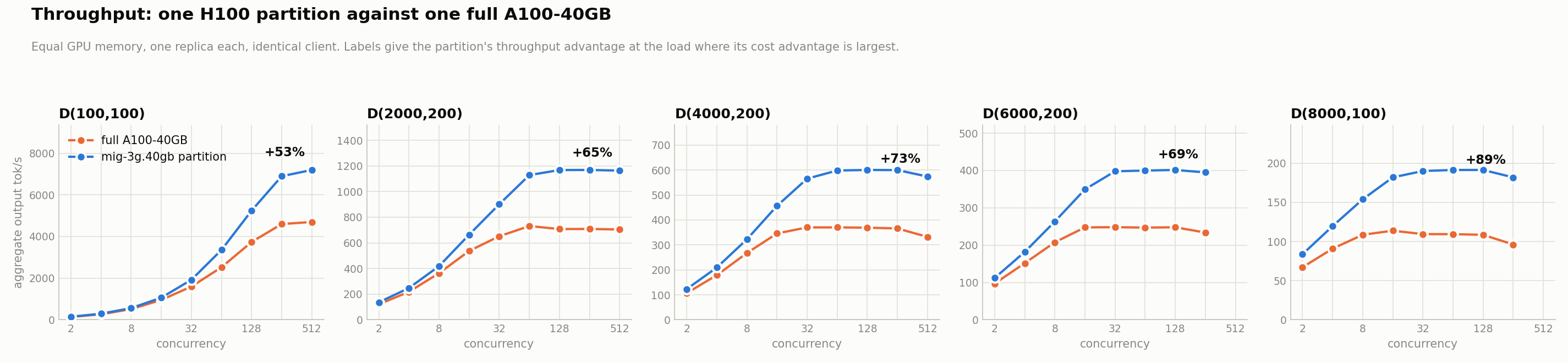
Figure 1: Aggregate output tokens per second for one mig-3g.40gb partition of an H100 against one full A100-40GB, across five traffic shapes and a concurrency ladder from 2 to 512
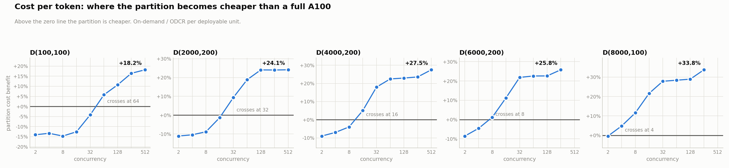
Figure 2: Partition cost benefit per million output tokens against concurrency for the same five traffic shapes
Four things stand out.
- The partition is faster everywhere – It delivered more output tokens per second in every scenario at every concurrency, by 53 percent to 89 percent at the load where each scenario’s cost benefit is largest, and lower inter-token latency in every one too, by 8.9 percent to 42.1 percent. The gap widens with load.
- Time to first token is lower in every case, by 5.6 percent to 47.5 percent.
- On cost it’s 18–34 percent cheaper per million output tokens, above a crossover that moves earlier as prompts lengthen. Concurrency 64 for 100-token prompts, 4 for 8,000-token prompts. Below the crossover the whole A100 is the cheaper unit. These prices are all on-demand, which at the time of analysis were measured as $25.251286 per hour for an
ml.p4d.24xlargeand $63.296000 per hour for anml.p5.48xlargein the US West (Oregon) AWS Region. Purely for our own analysis, we derived the unit cost by dividing the whole-instance cost by the number of units on it: 8 on the p4d, and 16 on the p5, where our partition is half of a GPU. - At the top of the ladder on long-context traffic, the A100 stopped serving. On both the 6,000- and 8,000-token workloads it failed a third to a half of its requests against a serving-path deadline, while the partition failed none. That is why those two panels end earlier than the rest.
Treat this as a case-by-case comparison, not a verdict. The useful mental model is to regard the available GPU fractions as GPU types in their own right. List them alongside whole accelerators, work out what your traffic actually demands of compute and of memory, and compare them on your own workload. For high-concurrency, long-input traffic the partition won on both performance and cost here. For short-input or low-concurrency workloads the whole A100 remained cheaper. Partitioning isn’t a one-size-fits-all answer. It gives you more sizes to choose from, so you can pick the one that fits your workload.
What to know before you commit to a layout
Partitioning changes the shape of an endpoint, and a few properties are worth understanding before you design one.
A component’s partition type is fixed for the life of that component. Moving a model to a different profile means creating a new component. Changing the endpoint’s carve means a new endpoint and a traffic migration, because updating an endpoint configuration doesn’t re-carve hosts that are already running. This makes partitioning a good fit for a stable portfolio and a poor one for a mix you reshuffle daily.
A requested profile has to exist in the endpoint’s layout. There is no fallback to a whole accelerator, so a component asking for a profile the variant didn’t declare is rejected.
Partitioning applies to real-time inference on inference component endpoints. Serverless endpoints and heterogeneous instance pools aren’t supported, and asynchronous invocation cannot address an inference component, so async workloads are out of scope.
You’re billed for the full GPU instance, as you are today. Partitioning raises how much of that instance you can use. It doesn’t change its hourly price.
Finally, a model that genuinely needs a full accelerator, or more than one, should keep having one. No partition spans accelerators.
Supported instances and Regions
GPU partitioning is available on the P4d, P5, G7, and G7e instance families. Support is at the family level, so smaller sizes within a family are covered.
It’s available in the following AWS Regions: US East (N. Virginia), US East (Ohio), US West (Oregon), Asia Pacific (Singapore), Asia Pacific (Tokyo), Europe (Frankfurt), and Europe (Ireland).
Instance availability varies by Region, so confirm that your chosen instance type is offered in your Region and that you have endpoint usage quota for it.
Getting started
To partition a GPU endpoint, work out the memory and compute each of your model’s needs, pick the profiles that fit, declare a layout on your endpoint configuration, and deploy each model as an inference component that requests a profile from that layout. Nothing about how you invoke your models changes.
For the API reference, the full profile tables for each instance family, and a step-by-step walkthrough, see GPU partitioning in the Amazon SageMaker AI Developer Guide.
To try it yourself, run the GPU partitioning sample notebook, which deploys several models onto partitions of a single GPU endpoint.
The broader change is worth keeping in mind as you plan capacity. Every supported accelerator is now several sizes rather than one. Whether a partition of a newer GPU or a whole accelerator of an older one is the right unit for a given model is no longer a question you need to answer by rounding up. It’s one you can measure.