AWS Machine Learning Blog
Building an Autonomous Vehicle, Part 4: Using Behavioral Cloning with Apache MXNet for Your Self-Driving Car
In the first blog post of our autonomous vehicle series, you built your Donkey vehicle and deployed your pilot server onto an Amazon EC2 instance. In the second blog post, you learned to drive the Donkey car, and the Donkey car learned to self-drive. In the third blog post, you learned about the process of streaming telemetry from the Donkey vehicle into AWS using AWS IoT.
In this blog post, we will deep dive on the Deep Learning that enables your car to drive, and introduce the concept of behavioral cloning with Convolutional Neural Networks (CNNs). CNNs have emerged as the state-of-the-art modeling technique for computer vision tasks, including answering questions that your car may encounter, such as, “Is there a track or a cone in front of me?”
1) Build an Autonomous Vehicle on AWS and Race It at the re:Invent Robocar Rally
2) Build an Autonomous Vehicle Part 2: Driving Your Vehicle
3) Building an Autonomous Vehicle Part 3: Connecting Your Autonomous Vehicle
4) Building an Autonomous Vehicle Part 4: Using Behavioral Cloning with Apache MXNet for Your Self-Driving Car
Training data setup for Donkey on P2
We have already walked you through the details on how to run the training in blog post 2. But let’s recap the key steps and commands here:
- Copy the data from the Pi to our Amazon EC2 instance:
- Kick off the training process:
- Copy the trained model back to the Pi:
Behind the scenes of the model
In this section, I’ll discuss what the model learns and how it can drive on its own. The current donkey build uses Keras as its default deep learning framework. AWS is in the process of adding support for other frameworks like Apache MXNet, Gluon, and PyTorch. We will use Apache MXNet in this blog post to dive deeper in to the inner workings of the model that enables self-driving. As previously mentioned, we use a technique called as behavioral cloning to enable self-driving of the car. The model essentially learns to drive based on the training data, which was collected by driving around the track. It’s essential that most of the data is “clean”, that is, we don’t have a lot of images in the training data where the car isn’t on the track or making wrong turns, given that our objective is to stay on the track. Just like the human driver who controls the steering to keep the car on track, we will build a model that will determine the steering angle given the current scenario, which leads us to model the problem as “what’s the steering angle we need to take given the input image?”. Real driving scenarios are more complicated with additional components like acceleration and transmission gears. We keep it simple to start with by fixing the throttle to some percentage for the car to drive. In practice, we have found that for spare training data 25-30% throttle has proven to be the best speed for the donkey car.
To make this happen we use a Deep Learning technique called Convolutional Neural Networks (CNNs). CNNs have emerged as the de facto networks for computer vision problems. CNNs are made of convolutional layers, where each of their nodes is associated with a small window called a receptive field. This allows us to extract local features in the image. Questions like, “is there a track or a person in the image?” can be computed using these local features computed earlier. You can find more detailed explanation of how CNNs work here.
Dataset
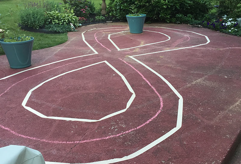
For this blog post I’ll use a dataset that we collected by driving the car for roughly 15 minutes around the track. As mentioned, we did a cleaning pass and discarded images where the car was clearing out of the track. The donkey software already provides a browser-based UI to delete “bad” images (command: donkey tubclean <folder containing tubs>). The dataset of images of the car driving on a track similar to this is available here.
Building the CNN model
Using the im2rec.py tool we convert the image dataset in to binary files for faster processing. To learn more about Apache MXNet internals visit the tutorial page.
Given that we need to determine the angle the car needs to steer, we use a linear regression output layer with a single output. To evaluate the progress on how the training process proceeds we can use mean absolute error (MAE) as the evaluation metric. Since the distance between angles is interpretable in the Euclidean system, MAE is a good metric to optimize our loss.
Training the model
The binary files are made available in our S3 bucket to train on.
Evaluation and simulator
Now that we have trained a model, we can deploy it on the car and take it for a spin. A low MAE error on our validation set is a good indication that our model is well trained and generalized. However, it would be great to have a better idea how the car would do before we deploy visually. To help with that I present a simulator to see how a car might drive on the track.
Conclusion
This concludes our autonomous vehicle series. We hope to see you at the re:Invent Robocar Rally 2017, a two-day hackathon for hands on experience with deep learning, autonomous cars, and Amazon AI and IoT services. We encourage you to continue following Donkey Car and to join the community!