AWS for Industries
Novartis AG uses Amazon OpenSearch Service K-Nearest Neighbor (KNN) and Amazon SageMaker to power search and recommendation (Part 3/4)
September 8, 2021: Amazon Elasticsearch Service has been renamed to Amazon OpenSearch Service. See details.
This is the third post of a four-part series on the strategic collaboration between AWS and Novartis AG, where the AWS Professional Services team built the Buying Engine platform.
In this series:
- Part 1: How Novartis AG brought SMART into Smart Procurement with AWS Machine Learning
- Part 2: Novartis AG uses Amazon SageMaker and Amazon Neptune to build and enrich a knowledge graph using BERT
- Part 3: Novartis AG uses Amazon OpenSearch Service K-Nearest Neighbor (KNN) and Amazon SageMaker to power search and recommendation (this post)
- Part 4: Demand Forecasting with Amazon SageMaker and GluonTS at Novartis AG
This post focuses on the search and recommendation components of the Buying Engine, specifically on the usage of Amazon OpenSearch Service (successor to Amazon Elasticsearch Service) and its k-nearest neighbors (KNN) functionality, in addition to Amazon SageMaker. With these services, Novartis built a scalable search and recommendation engine powered by machine learning.
Project motivation
The Novartis Buying Engine platform is meant to help Novartis employees in making informed buying decisions, which makes search and discovery capabilities key components of the project. Users must be able to select the most appropriate product from a catalog of over 2 million items across a wide variety of vendors, taking into account price, product properties, and other details.
The goal of the search component is to provide users with the ability to find the most relevant products using free text. Classic search mechanisms depend heavily on key-word matching and ignore the lexical meaning or query’s context. To provide a robust search experience, we trained a natural language model and incorporated it within the search engine using the KNN functionality of Amazon ES.
The recommendation component, on the other hand, provides a mechanism for users to continue the discovery journey on product detail pages. Since purchase history is not always available, we explored the idea of using the same KNN functionality in the search engine to also serve recommendations.
In this blog post, we provide technical guidelines on building a search and recommendation engine for data scientists working on similar challenges. We provide guidance on how to:
- Train a custom language model using Amazon SageMaker Object2Vec to generate textual embeddings for each catalog product
- Visualize the embeddings using TensorBoard Embedding Projector
- Set up a cluster using an Amazon OpenSearch Service domain and populate it with embeddings in addition to the catalog data (title, description price, product properties, etc.)
- Conclude with a mechanism to combine key word and KNN functionality to perform search and recommendation queries
Setting up
- Create an Amazon S3 bucket. This will be used throughout the notebooks to store files generated by the examples.
- Create a SageMaker notebook instance. Please observe the following:
-
- The execution role must be given an additional permission to read/write from the S3 bucket created in step 1.
- If you put the notebook instance inside a Virtual Private Cloud (VPC), make sure that the VPC allows access to the public Pypi repository and
aws-samples/repositories - Attach the Git repository Amazon SageMaker KNN Search to the notebook, as shown in the following screenshots.


Generating textual embeddings using catalog data
First, generate textual embeddings for each product within the catalog data. Textual embeddings are a mathematical representation of words (and text in general) through a high-dimensional vector containing actual numbers.
SageMaker is a fully managed service that provides every developer and data scientist with the ability to build, train, and deploy machine learning models quickly. Its built-in model Object2Vec is a highly customizable multi-purpose algorithm that can learn low dimensional dense embeddings of high dimensional objects. This section covers data preparation, training, and inference.
Data overview and preparation
For this post, we are using the Amazon reviews dataset, we will only make use of the product category and title (which is we consider as the product’s short description). For demo purposes we focus have picked four product categories and about 400,000 products.
Each item contains a unique identifier, title description, and product category among other product properties. The following table shows a representation of the dataset:

The end goal is to project user queries and catalog products into a high dimensional space where the distance of their representation correlates with their conceptual meaning. You need a labeled dataset to learn these embeddings using Object2Vec, as the algorithm is a supervised learner.
This labeled dataset is constructed using the catalog data based on the following hypothesis: A positive pair (label=1) consists of two products from the same category and a negative pair (label=0) consists of two products from different categories. The following figures explains two sample pairs that are passed through the network:

The data used in this example is small for demo purposes, but in the Novartis project, we used a large dataset with millions of products and thousands of categories. Creating all possible combinations of positive and negative pairs would have produced an exponential number of pairs. To solve this issue while still representing the overall dataset, we defined the number of data points to train on beforehand and used a stratified sampling technique based on the distribution of categories when generating the pairs.
Training with the SageMaker built-in Object2Vec algorithm
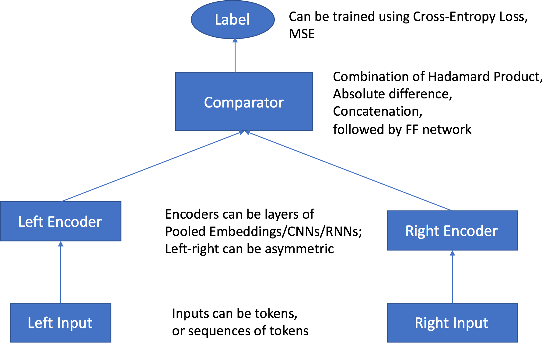
During training, the Object2Vec algorithm reads a list of inputs. Each input is pair object (a, b) and a label (L=0/1). The pairs (a, b) are passed through the left and right encoders respectively, which generates a vector representation for each (i.e. embeddings).
These two embeddings are compared using the Comparator layer producing a predicted label (P_L=0/1). The algorithm then compares the ground truth label (L=0/1) and predicted label (P_L=0/1), and propagates the feedbacks through the network to update the parameters.
Use the SageMaker SDK to create an Estimator around the Object2Vec built-in algorithm. Define the hyperparameters and the data input channels as:
To initialize the embeddings of common words that will be present in your data, use Glove embeddings pre-trained on the Common Crawl dataset containing 840B tokens. (See GloVe: Global Vectors for Word Representation.) For words that are very specific to the pharmaceutical industry or to vendors within the catalog, the initialization is random.
Do this by specifying a third input channel called “auxiliary,” where you pass the pre-trained token embedding file. Also, add the following two hyperparameters:
Now, apply the following hyperparameters to the estimator and launch the SageMaker training job:
Quantitative and qualitative evaluation
During training, you evaluate your model using the built-in metrics of Object2Vec for classification (i.e. Softmax). This gives an idea of how well the model did in learning to classify two semantically similar descriptions. These metrics can be extracted from the training job once completed:
You can also evaluate your embeddings using a qualitative analysis. Randomly sample a subset of embeddings generated from the previous section and visualize them using the TensorBoard Embedding Projector. This functionality lets you project high dimensional embeddings in a 2D/3D space using dimension reduction techniques like PCA or t-SNE.
TensorBoard typically reads data and metadata from a logs directory that you specify and in which you save checkpoints, metadata, etc. For this example, use the following code to read embeddings from a CSV file:
Then, create the logs directory and save the necessary information in it (i.e. checkpoints, metadata).
While specifying the log directory where the metadata and checkpoints are saved, open a terminal and launch run the following command:
You can now access TensorBoard using the proxy number communicated in the terminal:
In the following figure, each point in the space represents an embedding/product. You can see multiple clusters being formed (mainly four).
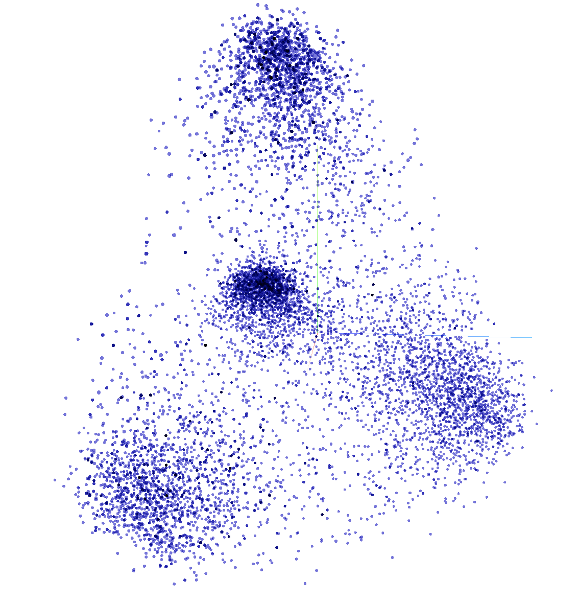

For example, when zooming on the cluster in the low left part of the figure you can see a concentration of furniture-related products. This allows you to visually evaluate your embeddings. The more clusters that are formed, the more your Object2Vec model can differentiate and separate categories.
A machine learning-powered engine
This section covers how to create an engine that combines key word search and KNN-based search using embeddings. This involves configuring an Elasticsearch cluster and ingest enriched data (catalog data+embeddings) and performing free text search queries. Then, we cover how this engine can also be used for recommendation.
Setting up the Amazon Elasticsearch Service domain using KNN settings
First, set up an Opensearch cluster. For instructions, see Creating and Managing Amazon OpenSearch Service Domains. You can also use the CloudFormation template provided within the Git repository Amazon SageMaker KNN Search.
Once the Elasticsearch cluster is set up, create an index to store the catalog data and the embeddings. The index settings must be configured beforehand to enable the KNN functionality using the following configuration:
This example uses the Python Elasticsearch client to communicate with the Elasticsearch cluster and create an index to host our data.
Ingesting enriched data into Amazon ES
Once the training finishes, create a SageMaker model directly from the training job name. Make sure to specify the environment variable ‘INFERENCE_PREFERRED_MODE’ and set it to ‘embedding’ so that embeddings are outputted instead of classification values during inference.
The next step is to add these embeddings into the catalog. To ensure a robust and scalable solution, you can put an automated ingestion pipeline in place, as illustrated in the following picture:

The pipeline makes use of SageMaker Batch Transform job to perform the predictions using the preceding model, in addition to SageMaker processing jobs that take care of data processing. Once the data is enriched, an event is triggered using Amazon CloudWatch events calling an AWS Lambda function that will first store the data in Amazon DynamoDB. Finally, a DynamoDB stream is set up to stream the data to Amazon ES.
A mechanism to combine key word and KNN queries
As mentioned earlier, embeddings are created for product catalog data to enhance the search results and go beyond key-word search. To perform a simple key word search query, do the following:
The results of this query will be ordered based on the default scoring mechanisms of Amazon ES, which use a probabilistic ranking framework called BM-25 (TF-IDF) to calculate relevance scores. BM 25 (TF-IDF) multiplies the number of occurrences of a query term by the inverse of the count of that term in the corpus of documents. It also uses various parameters that normalize for length, discount for common terms, etc.
KNN for Amazon ES lets you search for points in a vector space and find the “nearest neighbors” for those points by Euclidean distance or Cosine similarity.
Deploy a SageMaker Endpoint using the same SageMaker model that was used during the inference stage. When receiving a query from the user, the query is transformed into a list of tokens using our vocabulary (i.e. mapping of words to IDs) and sends it as a payload to the Object2vec Endpoint. This gives you a vector of numbers (i.e. the embeddings). Then, use the embedding of the query to perform a KNN search query:
Let’s take a look at the results of a simple query, like “office.” The keyword approach returns the following products:
Only products with the keyword “office” came up. On the other hand, the embedding approach returns the following results:
Relevant products are still being returned, but now with the addition of more diverse ones related to the word “office” (e.g. “computer”, “desk”).
To get the best keyword matching and embeddings, combine both approaches. The following figure and steps illustrate how to do so:

- Using the should parameter, you can incorporate two search queries and return the ranked result based on a combined score from both.
- The first search query performs keyword matching, with fuzzy matching enabled on a pre-defined list of search fields.
- The boost_search parameter is used to give a weight to the results of the first search query to show how important it is.
- The second search query performs a KNN type of query by providing the embedded textual query in the “vector” section.
- The boost_embeddings parameter is used to give a weight to the results of the second search query to show how important it is.
- The filter_list is used to filter the results based on the user’s selected filters. For example, (color=”blue”).
- The page_size and page_from are used to control the number of results we return and enable pagination.
Performing real-time recommendation requests
When building a customer-facing catalog platform, it takes time to collect user buying patterns to build a robust recommendation system. On the other hand, content-based recommendation systems require mainly information about the products.
As textual embeddings were already computed for each product, this information can determine the k-most similar products in the following steps:
- A user browsing the details page of “product A” will trigger the recommendation component.
- The recommendation component will extract the embeddings of “product A” from the database, as it now contains both product information and textual embeddings.
- A search API call is made using the extracted embeddings, resulting in a list of the k-nearest neighbors and thus, similar products.
Following this mechanism, you can use the same machine learning engine for both search and recommendation requests.
Cleaning Up
When you finish this exercise, remove your resources with the following steps:
- Delete your notebook instance and the endpoint created.
- Optionally, delete registered models.
- Optionally, delete the SageMaker execution role.
- Optionally, empty and delete the S3 bucket, or keep whatever you want.
Summary
The AWS Professional Services team provides assistance through a collection of offerings which help customers achieve specific outcomes related to enterprise cloud adoption. Along with the Novartis team, we were able to build an end-to-end solution to enrich catalog data and build a machine learning-powered search and recommendation engine. This enables end users to search and discover products in an accurate and informative manner, helping them make the best buying decisions.
Get started today! You can learn more about SageMaker and kick off your own machine learning solution by visiting the Amazon SageMaker console.
AWS welcomes your feedback. Feel free to leave us any questions or comments.
Many thanks to the Novartis team who worked on the Buying Engine project. Special thanks to following, who contributed to this blog post:
- Srayanta Mukherjee: Srayanta is Director of Data Science on Novartis CDO’s Data Science & Artificial Intelligence team. He was the data science lead during the delivery for the Novartis Buying Engine.
- Preeti Chauhan: Preeti is Associate Director of Data Science on Novartis CDO’s Data Science & Artificial Intelligence team. She was a co-lead for the delivery of Discovery and Decisions system for the Novartis Buying Engine.
- Megha Hada: Megha is Senior Expert Data Scientist on Novartis CDO’s Data Science & Artificial Intelligence team. She was a co-lead for the delivery of Discovery and Decisions system for the Novartis Buying Engine.