AWS for Industries

Demand Forecasting using Amazon SageMaker and GluonTS at Novartis AG (Part 4/4)

This is the fourth post of a four-part series on the strategic collaboration between AWS and Novartis AG, where the AWS Professional Services team built the Buying Engine platform.

In this series:

This post focuses on the demand forecasting component in the Buying Engine, specifically on the usage of Amazon SageMaker and MXNet GluonTS library. SageMaker is a fully managed service that provides every developer and data scientist with the ability to build, train, and deploy machine learning models quickly. The combination with GluonTS unlocks state-of-the-art, deep learning-based forecasting algorithms and streamlines the processing pipelines, which shorten the time from ideation to production.

Project motivation

Holistic optimization of the procurement chain for all goods and services is a core building block as Novartis works towards its larger goal to build an automated replenishment engine driven by demand and forecasting. Being able to predict demand for each Stock Keeping Unit (SKU) at particular geography several months in advance allows Novartis to make faster data-driven decisions, plan better, and negotiate contracts and discounts as well as save costs.

The motivation to use MXNet GluonTS was that it provides a toolkit to work with time series data in a simpler fashion, and many state-of-the-art custom models to be trained and benchmarked under the same API. We were able to create a baseline model, train DeepAR and DeepState, as well as experiment with other models much quicker with only parametric changes to the code.

This reminder of this blog guides you through the following steps: (1) notebook setup; (2) prepare dataset; (3) training; and (4) inference.

Notebook Setup

  1. Create an Amazon S3 bucket. This will be used throughout the notebooks to store files generated by the examples.
  2. Create a SageMaker notebook instance. Please observe the following:
    1. The execution role must be given an additional permission to read/write from the S3 bucket created in step 1.
    2. If you put the notebook instance inside a Virtual Private Cloud (VPC), make sure that the VPC allows access to the public Pypi repository and
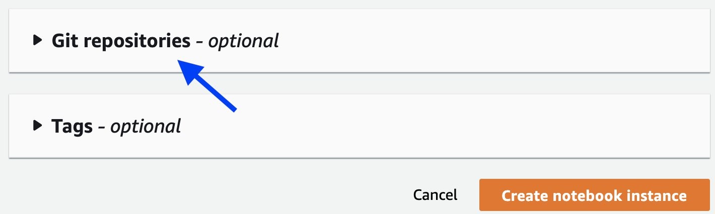
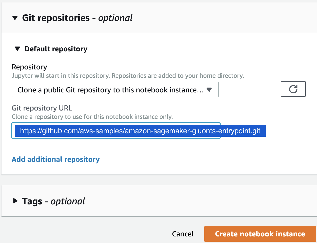
 aws-samples/ repositories.
    3. Attach the Git repository amazon-sagemaker-gluonts-entrypointto the notebook, as shown in the following screenshots, then click the Create notebook instance

When the notebook instance is ready, you can work with the familiar JupyterLab interface with the workspace defaults to the amazon-sagemaker-gluonts-entrypoint folder. The next screenshot illustrates the key content in the folder.

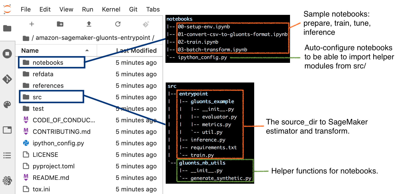
To complete this step, open notebooks/00-setup-env.ipynb and make sure the selected kernel is conda_mxnet_p36. Run this notebook to install additional modules required by subsequent steps, and to generate a synthetic data in the CSV format.

Prepare dataset in GluonTS format

Out of 3 million products in the Novartis Buying Engine product catalog, a few thousands are high-frequency SKUs, each of which is represented as a time series describing historical demand over the last several years. For the purpose of this blog, we describe how we used deep learning models with GluonTS to generate weekly forecasts for 3-months, and daily forecasts for 14-days in advance.

Let’s convert the CSV data to the GluonTS format. We start by using ListDataSet to hold the train and test splits. Then, we utilize GluonTS’s TrainDataSets and save_datasets() APIs to save those ListDataSet to files. The TrainDataSets provides an abstraction of a container of metadata, train split, and test split. The TrainDataSets will later on become a single data channel for a SageMaker training job. Having metadata for datasets is crucial for reproducibility and to be able to track what a dataset is about and how it was created, especially for prolonged usage across cross-team collaboration.

The following stanza shows how the APIs work. Please refer to notebooks/01-convert-csv-to-gluonts-format.ipynb in the sample Git repository aws-samples/amazon-sagemaker-gluonts-entrypoint for the complete code. First, use ListDataSet to convert your Pandas dataframe to an in-memory structure that’s compatible with GluonTS.

def encode_SKU(skus):
    # creates a dictionary of SKU to integer mapping, e.g. "product ABC": 1
    return {c:i for i,c in enumerate(skus)}


def df2gluonts(
    df,
    cat_idx,
    fcast_len: int,
    freq: str = "D",
    ts_id: Sequence[str] = ["sku"],
    static_cat: Sequence[str] = ["sku"],
    item_id_fn: Callable = None,
) -> None:
    '''
    Converts time-series data into GluonTS format
    Args:
        df: pd.DataFrame containing time-series data
        sku_idx: dictionary of SKU indexes
        fcast_len: forecast length, by default 12 weeks
        freq: time-series data frequency, e.g. W weekly, D daily
        ts_id: list of time-series ID/s, e.g. sku, [sku, cost-center] 
        static_cat: one or more columns for static categories
        item_id_fn: item ID representation for plots
    Returns:
        ListDataset: Converted dataset backed by list of dicts
    '''
    
    # List that contains all time-series in dataset.
    # Each time-series record should be a dictionary mapping strings to values
    # For instance: {"start": "2014-09-07", "target": [0.1, 0.2]}.
    # See also: https://ts.gluon.ai/examples/extended_forecasting_tutorial/extended_tutorial.html#1.3-Use-your-time-series-and-features
    data_iter = [] 
    
    # Build the payload: the following loop transforms the given df into
    # dict mapping as described above and store in data_iter.
    for item_id, dfg in df.groupby(ts_id, as_index=False):
        if len(ts_id) < 2:
            item_id = [item_id]

        if fcast_len > 0:
            # Train split exclude the last fcast_len timestamps
            ts_len = len(dfg) - fcast_len
            target = dfg['y'][:-fcast_len]
        else:
            # Test split include all timeseries. During backtesting,
            # gluonts will treat the fcast_len as groundtruth.
            target = dfg['y']
 
        feat_static_cat = []
        for col in static_cat:
            # Construct all static category features of current timeseries.
            assert dfg[col].nunique() == 1
            sku_value = dfg[col].iloc[0]
            # Encode sku to zero-based number for feat_static_cat.
            feat_static_cat.append(sku_idx[col][sku_value])

        if item_id_fn is None:
            # NOTE: our sm-glounts entrypoint will interpret '|' as '\n'
            # in the plot title.
            item_id = '|'.join(item_id)
        else:
            item_id = item_id_fn(*item_id)

        data_iter.append({
            'start': dfg.iloc[0]['x'],
            'target': target,
            'feat_static_cat': feat_static_cat,
            'item_id': item_id
        })

    # Finally we call gluonts API to convert data_iter with frequency of 
    # the observation in the time series
    data = ListDataset(data_iter, freq = freq)
    return data

# Zero-based SKU encoding.
# TS is a pd.DataFrame that contains time series for each SKU,
# where all timeseries have the same frequency.
sku_inverted_idx = {'sku': encode_SKU(ts['sku'].unique())}

# Train split
train_data = df2gluonts(
    ts,
    sku_inverted_idx,
    fcast_len=fcast_length,  # Exclude the final fcast_len timestamps.
    freq=freq, 
    ts_id=['sku'],
    static_cat=['sku']
)

# Test split
test_data = df2gluonts(
    ts,
    sku_inverted_idx,
    fcast_len=0,  # Whole timeseries; the last fcast_length timestamps are groundtruth.
    freq=freq,
    ts_id=['sku'],
    static_cat=['sku']
)

Next, we’ll manage the train split, test split, and an additional metadata as a single construct called TrainDataSets, then save to local disk. See the next stanza.

gluonts_datasets = TrainDatasets(
    metadata=MetaData(
                freq=freq,
                target={'name': 'gr'},
                feat_static_cat=[
                    CategoricalFeatureInfo(name=k, cardinality=len(v)+1)   # Add 'unkown'.
                    for k,v in sku_inverted_idx.items()
                ],
                prediction_length = fcast_length
    ),
    train=train_data,
    test=test_data
)

# Setting `overwrite=True` means:
# - rm -fr path_str, then
# - mkdir path_str, then
# - write individual files.
local_path=f'../../data/processed/{dataset_name}'
save_datasets(
    dataset=gluonts_datasets,
    path_str=local_path,
    overwrite=True
)

# Save also our indexes
with open(Path(local_path) / 'metadata' / 'sku.json', 'w') as f:
    json.dump(sku_inverted_idx, f)

You can then upload the dataset to S3.

Training

Please refer to notebooks/02-train.ipynb for the complete code of model training and tuning. Here, we focus straightaway on hyperparameter tuning. For additional information, see SageMaker documentations on model training and model tuning.

The following stanza shows a helper function that starts a tuning job. Each tuning job spawns one or more training jobs, and each training job uses the same entrypoint train script from the sample Git repository. In our example, training jobs utilize the Managed Spot Training for Amazon SageMaker, a feature based on Amazon EC2 Spot Instances that will help you lower ML training costs by up to 90% compared to using on-demand instances in SageMaker.

# Metric emitted by each training job. The entrypoint script may emit even
# more metrics, however this example captures only a few.
metric=[
    {"Name": "train:loss", "Regex": r"Epoch\[\d+\] Evaluation metric 'epoch_loss'=(\S+)"},
    {"Name": "train:learning_rate", "Regex": r"Epoch\[\d+\] Learning rate is (\S+)"},
    {"Name": "test:abs_error", "Regex": r"gluonts\[metric-abs_error\]: (\S+)"},
    {"Name": "test:rmse", "Regex": r"gluonts\[metric-RMSE\]: (\S+)"},
    {"Name": "test:mape", "Regex": r"gluonts\[metric-MAPE\]: (\S+)"},
    {"Name": "test:smape", "Regex": r"gluonts\[metric-sMAPE\]: (\S+)"},
    {"Name": "test:wmape", "Regex": r"gluonts\[metric-wMAPE\]: (\S+)"},
]

def create_tuning_job(objective_metric_name, estimator_hp, tuner_hp, metric, role, sess, max_jobs=10):
    # Define the estimator that uses the entrypoint train script 
    estimator = MXNet(entry_point='train.py',
                      source_dir='../../src/entrypoint',
                      framework_version='1.6.0',
                      py_version='py3',
                      role=role,
                      train_instance_count=1,
                      train_instance_type='ml.c5.4xlarge',
                      train_max_run=24*60*60,
                      train_use_spot_instances=True, # using spot instances allows better cost savings
                      train_max_wait=24*60*60,
                      sagemaker_session=sess,
                      hyperparameters=estimator_hp,
                      metric_definitions=metric,
    )

    tuner = HyperparameterTuner(
                estimator,
                objective_metric_name,
                tuner_hp,
                metric,   # Also needed for custom algo. (i.e., entrypoint train script).
                objective_type='Minimize',
                max_jobs=max_jobs,
                max_parallel_jobs=1)
    return tuner

def get_ts():
    # get timestamp
    return strftime("%y%m%d-%H%M%S", gmtime())

We can then submit multiple tuning jobs, one for a different algorithm. Our example of a single entrypoint train script supports four different models: DeepAR, DeepState, DeepFactor, and Transformer. All these algorithms are already implemented in GluonTS; hence, we simply tap into it to quickly iterate and experiment over different models. Please refer to src/entrypoint/train.py on the implementation details. For more details of the four algorithms, and additional algorithms not covered here, please refer to gluonts model documentation.

The following stanza show to submit a Hyperparameter Tuning job for DeepAR (please refer to the notebook for the DeepState example). The key novelty of the entrypoint train script is to passthrough the hyperparameters it receives as command line arguments, directly to the specified estimator, yet the entrypoint train script does not need to explicitly declare all those hyperparameters in its body. The passthrough mechanic simplifies the overhead of supporting new estimator in future.

[SFG17] Salinas, David, Valentin Flunkert, and Jan Gasthaus. “DeepAR: Probabilistic forecasting with autoregressive recurrent networks.” arXiv preprint arXiv:1704.04110 (2017).

# Create tuner
tuner_deepar = create_tuning_job(
    objective_metric_name='test:wmape',
    # Fixed hyperparameters, i.e., same for all training jobs.
    estimator_hp={
        # Hyperparameters for the script
        'plot_transparent': 0,
        'num_samples': 1000,
        'y_transform': 'log1p',

        # Select estimator
        'algo': 'gluonts.model.deepar.DeepAREstimator',

        # Hyperparameters for glounts.model.deepar.DeepAREstimator.
        # See:  https://gluon-ts.mxnet.io/api/gluonts/gluonts.model.deepar.html
        #
        # Script will passthrough these to DeepAREstimator.__init__().
        'prediction_length': fcast_length,
        'use_feat_static_cat': 'True',
        'cardinality': json.dumps(cardinality),
        'cell_type': 'gru',

        # Special syntax to say Trainer(epochs=...)
        'trainer.__class__': 'gluonts.trainer.Trainer',
        'trainer.epochs': 300,
    },

    # Tunable hyperparameters, i.e., may vary across training jobs.
    # Script will passthrough these to DeepAREstimator.__init__().
    tuner_hp={
        "context_length": CategoricalParameter([fcast_length, fcast_length*2]),
        "cell_type": CategoricalParameter(["lstm", "gru"]),
        "num_cells": IntegerParameter(30, 100),
        "num_layers": IntegerParameter(2, 5),
        # Special syntax to say Trainer(learning_rate=...)
        "trainer.learning_rate": ContinuousParameter(1e-6, 1e-3, scaling_type='Logarithmic'),
    },

    metric=metric,
    role=role,
    sess=sess,
    max_jobs=5)

# Start hyperparameter tuning job.
tuner_deepar.fit(
    data_channels,
    job_name='w-da-'+get_ts(),
    include_cls_metadata=False
)

The tuning job runs, and on completion will show the best training job. You can follow through the best training job, then go to the output location, which contains two files: model.tar.gz and output.tar.gz. The former is the model artifact, the later contains the training information produced by our entrypoint train script.

To facilitate rapid experiment, the entrypoint train script outputs all the test metrics, and in addition, the test forecasts, and automatically render the plots of forecast-vs-groundtruth as montages and as individual charts. As such, data scientists can simply download the output and start making post-mortem analysis and reasoning without having to write additional boiler-plate, tedious codes. When data scientists observe interesting phenomena, then they can follow-up with further deep-dive. Please refer to src/entrypoint/train.py and src/entrypoint/gluonts_example/evaluator.py on the implementation details, in particular class MyEvaluator from src/entrypoint/gluonts_example/evaluator.py which customizes the GluonTS backtesting with the wMAPE metric and plots.

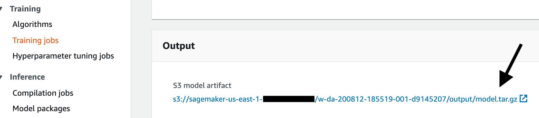
To download the training output from the console, first go to your training job, then scroll down until the Output section. Click the Amazon S3 model artifact to go to the S3 output area.

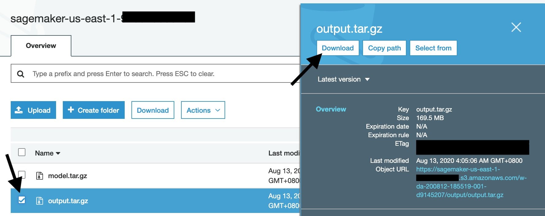
Once you download the output.tar.gz, open or extract it with your un-archiver, and you’ll see this structure:

output/
|-- agg_metrics.json           # Average metrics across all timeseries, multiple metrics.
|-- item_metrics.csv           # Metrics for each timeseries (i.e., SKU)
|-- mappings.csv               # Map SKU to individual plot
|-- plots
|-- |-- montages               #
|   |   |-- montage-0000.png   # - 10x10 for the 1st 100 SKUs
|   |   |-- montage-0001.png   # - 10x10 for the 2nd 100 SKUs
|   |   |-- ...
|   |   `-- montage-0033.png   # - 10x10 for the last 100 SKUs
|   `-- single                   
|       |-- 000.png            # The 1st SKU
|       |-- ...
|       |-- 3279.png           # The last SKU
|-- results.jsonl              # Forecast (of test split) of each SKUs
`-- daily-xxxx.csv             # One specific metric from agg_metrics.json, in csv form.

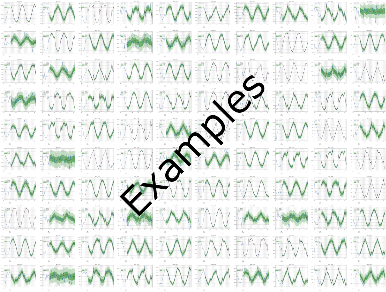
An example montage is shown here (zoomed-out for illustrative purpose). Each montage is 10×10 SKUs to provide bird-eye view for data scientists. The montage size is 5024 x 3766 pixels (100 dpi), thus 502 x 376 pixels per subplots.

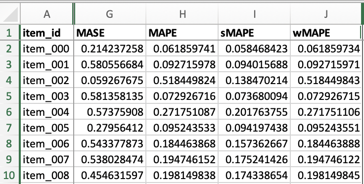
File item_metrics.csv contains the backtest performance of invidual SKUs, with an example shown below. Since forecasts are probabilistic, the specific metric of each SKU is the expected value of that metric out of a number of sample paths. Different metrics define their own expectation function, e.g., MASE, MAPE, sMAPE and our custom wMAPE use median, whereas MSE uses mean. Refer to get_metrics_per_ts() method of the MyEvaluator class in src/entrypoint/gluonts_example/evaluator.py for per-SKU wMAPE, and the get_metrics_per_ts() method in the gluonts.evaluation.Evaluator class for the built-in metrics.

File agg_metrics.json contains the aggregated backtest performance across all timeseries. Each metric may use a different function to aggregate per-SKU metrics. Our custom wMAPE uses mean as you can see from the get_aggregate_metrics() method of the MyEvaluator class in src/entrypoint/gluonts_example/evaluator.py). For the built-in metrics, please refer to get_aggregate_metrics() in the gluonts.evaluation.Evaluator class.

{
  ...
  "MASE": 0.41640195028553106,
  "MAPE": 0.20354243879215847,
  "sMAPE": 0.1513800091986696,
  ...
  "wMAPE": 0.9075764781422913
}

The rest of the training output files are self-explanatory, and we invite you inspect those files.

Create SageMaker model

Once you have decided on the best performing training job, you need to register the model artifact as a SageMaker model, as shown in the next stanza. The entrypoint inference script is located at  src/entrypoint/inference.py. Please refer to the first-half of notebooks/03-batch-transform.ipynb for the complete code example on registering your model artifact into a SageMaker model.

mxnet_model = MXNetModel(
        model_data=train_model_artifact,
        role=role,
        entry_point='inference.py',
        source_dir='../../src/entrypoint',
        py_version="py3",
        framework_version="1.6.0",
        sagemaker_session=sess,
        container_log_level=logging.DEBUG,
    )

Batch Inference

The following stanzas show detail implementations of the inference script src/entrypoint/inference.py, which will run on a SageMaker MXNet framework container. The script must adhere to the protocol defined here, hence our script provides  model_fn() and transform_fn().

First, take a look on its model_fn() .

def model_fn(model_dir: Union[str, Path]) -> Predictor:
    """Load a glounts model from a directory.

    Args:
        model_dir (Union[str, Path]): a directory where model is saved.

    Returns:
        Predictor: A GluonTS predictor.
    """
    predictor = Predictor.deserialize(Path(model_dir))

    # If model was trained on log-space, then forecast must be inverted before metrics etc.
    with open(os.path.join(model_dir, "y_transform.json"), "r") as f:
        y_transform = json.load(f)
        logger.info("model_fn: custom transformations = %s", y_transform)

        if y_transform["inverse_transform"] == "expm1":
            predictor.output_transform = expm1_and_clip_to_zero
        else:
            predictor.output_transform = clip_to_zero

        # Custom field
        predictor.pre_input_transform = log1p if y_transform["transform"] == "log1p" else None

    logger.info("predictor.pre_input_transform: %s", predictor.pre_input_transform)
    logger.info("predictor.output_transform: %s", predictor.output_transform)
    logger.info("model_fn() done; loaded predictor %s", predictor)

    return predictor

Next, take a look at transform_fn() shown in the next stanza. The key philosophy is to represent each timeseries as a JSON line, and this format is compatible with how SageMaker inference works (for both endpoints and batch transform), where each record must be a complete dataset. For text input format, each line corresponds to one record also known as time-series. It’s important to note that in the SageMaker inference construct, each record must be independent from each other, such that the model or inference script must not assume dependencies among different records.

Therefore, with text format, the GluonTS representations is suitable not only for GluonTS-based model, but also for other models. In fact, Novartis standardizes on this format across multiple models they’ve developed in-house, such as LSTM-on-PyTorch and XGBoost models. These different inference scripts share the same serialization and deserialization logics, and differ only in model_fn() and the prediction function. Please note that the format used in GluonTS differs with SageMaker first-party DeepAR: although both uses JSON lines, but the member keys are different. For readers looking for the inference input format of the SageMaker first party DeepAR, please check out this link.

def transform_fn(
    model: Predictor,
    request_body: Union[str, bytes],
    content_type: str = "application/json",
    accept_type: str = "application/json",
    num_samples: int = 1000,
) -> Union[bytes, Tuple[bytes, str]]:
    deser_input: List[DataEntry] = _input_fn(request_body, content_type)
    fcast: List[Forecast] = _predict_fn(deser_input, model, num_samples=num_samples)
    ser_output: Union[bytes, Tuple[bytes, str]] = _output_fn(fcast, accept_type)
    return ser_output


# Because of transform_fn(), we cannot use input_fn() as function name
# Hence, we prefix our helper function with an underscore.
def _input_fn(request_body: Union[str, bytes], request_content_type: str = "application/json") -> List[DataEntry]:
    """Deserialize JSON-lines into Python objects.

    Args:
        request_body (str): Incoming payload.
        request_content_type (str, optional): Ignored. Defaults to "".

    Returns:
        List[DataEntry]: List of GluonTS timeseries.
    """
    if isinstance(request_body, bytes):
        request_body = request_body.decode("utf-8")
    return [json.loads(line) for line in io.StringIO(request_body)]


# Because of transform_fn(), we cannot use predict_fn() as function name.
# Hence, we prefix our helper function with an underscore.
def _predict_fn(input_object: List[DataEntry], model: Predictor, num_samples=1000) -> List[Forecast]:
    """Take the deserialized JSON-lines, then perform inference against the loaded model.

    Args:
        input_object (List[DataEntry]): List of GluonTS timeseries.
        model (Predictor): A GluonTS predictor.
        num_samples (int, optional): Number of forecast paths for each timeseries. Defaults to 1000.

    Returns:
        List[Forecast]: List of forecast results.
    """
    # Create ListDataset here, because we need to match their freq with model's freq.
    X = ListDataset(input_object, freq=model.freq)

    # Apply forward transformation to input data, before injecting it to the predictor.
    if model.pre_input_transform is not None:
        logger.debug("Before model.pre_input_transform: %s", X.list_data)
        model.pre_input_transform(X)
        logger.debug("After model.pre_input_transform: %s", X.list_data)

    it = model.predict(X, num_samples=num_samples)
    return list(it)


# Because of transform_fn(), we cannot use output_fn() as function name.
# Hence, we prefix our helper function with an underscore.
def _output_fn(
    forecasts: List[Forecast],
    content_type: str = "application/json",
    config: Config = Config(quantiles=["0.1", "0.2", "0.3", "0.4", "0.5", "0.6", "0.7", "0.8", "0.9"]),
) -> Union[bytes, Tuple[bytes, str]]:
    """Take the prediction result and serializes it according to the response content type.

    Args:
        prediction (List[Forecast]): List of forecast results.
        content_type (str, optional): Ignored. Defaults to "".

    Returns:
        List[str]: List of JSON-lines, each denotes forecast results in quantiles.
    """

    # jsonify_floats is taken from gluonts/shell/serve/util.py
    #
    # The module depends on flask, and we may not want to import when testing in our own dev env.
    def jsonify_floats(json_object):
        """Traverse through the JSON object and converts non JSON-spec compliant floats(nan, -inf, inf) to string.

        Parameters
        ----------
        json_object
            JSON object
        """
        if isinstance(json_object, dict):
            return {k: jsonify_floats(v) for k, v in json_object.items()}
        elif isinstance(json_object, list):
            return [jsonify_floats(item) for item in json_object]
        elif isinstance(json_object, float):
            if np.isnan(json_object):
                return "NaN"
            elif np.isposinf(json_object):
                return "Infinity"
            elif np.isneginf(json_object):
                return "-Infinity"
            return json_object
        return json_object

    str_results = "\n".join((json.dumps(jsonify_floats(forecast.as_json_dict(config))) for forecast in forecasts))
    bytes_results = str.encode(str_results)
    return bytes_results, content_type

With the inference script, we’re now ready to perform batch inference. Do note that real-time inference via endpoints also leverage the same inference script, hence easing to real-time inferences in the future.

The next stanza is taken from notebooks/03-batch-transform.ipynb and shows how to programmatically start a batch transform job.

# Create transformer
bt = mxnet_model.transformer(
    instance_count=1,
    instance_type='ml.m5.large',
    strategy='MultiRecord',
    assemble_with='Line',
    output_path=bt_output,
    accept='application/json',
    max_payload=1,
    env={
        'SAGEMAKER_MODEL_SERVER_TIMEOUT': '3600',
    },
)

# Start batch transform job
bt.transform(
    data=bt_input,
    data_type='S3Prefix',
    content_type='application/json',
    split_type='Line',
    join_source='Input',
    output_filter='$',
    wait=False,
    logs=False,
)

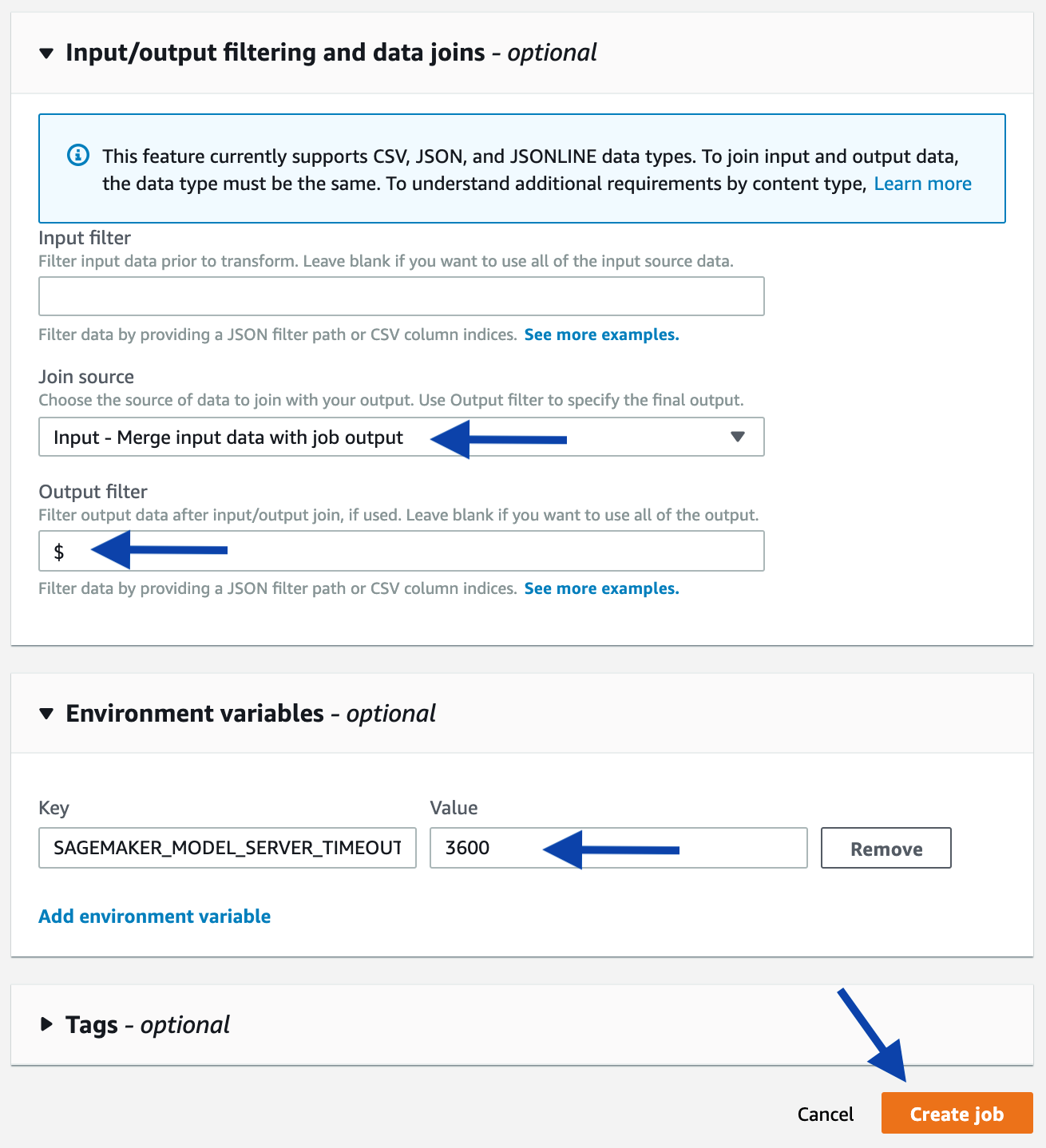
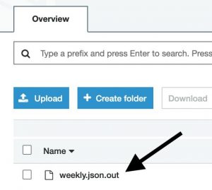
As an alternative, you can start a batch transform job using the console. Starting from the console of the selected model, click the Create batch transform job button. On the next page, provide the same information used in the above-mentioned programmatic example, such as the input path, output path, and input/output filter. Refer to the following screenshots as a guidance.

A forecast for an SKU will be a JSON structure in a JSON-line formatted file. You can quickly sample some results from the console: starting at the page of a completed Batch Transform job, follow the link to the output Amazon S3 location, then sample some lines.

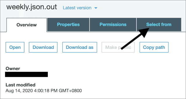
Next, we show an annotated output line, which denotes the forecast for a specific SKU. The comments facilitate understanding of the forecast output structure; however, they do not appear in the actual output file.

{
    # Output of Batch Transform
    "SageMakerOutput": {
        # Mean prediction, 12 timestamps (in this case: weeks)
        "mean": [57, 50, 63, 59, 63, 65, 71, 27, 69, 79, 78, 98],
        # Forecast at specific quantile, each quantile also has 12 length.
        "quantiles": {
            "0.1": [...],
            "0.2": [...],
            "0.3": [...],
            "0.4": [...],
            "0.5": [...],
            "0.6": [...],
            "0.7": [...],
            "0.8": [...],
            "0.9": [...],
        }
    },
    
    # These are the input, but re-included in the output using the
    # input-filter feature of Batch Transform. We do this to simplify
    # downstream tasks by providing all necessary information all
    # self-contained in the output files, rather than do extra steps
    # to join the output files with the input files.
    "feat_static_cat": [0], 
    "item_id": "XXXX",
    "start": "2017-04-02 00:00:00",
    "target": [...], 
}

Cleaning up

When you finish this exercise, remove your resources with the following steps:

  1. Delete your notebook instance
  2. Optionally, delete registered models
  3. Optionally, delete the SageMaker execution role
  4. Optionally, empty and delete the S3 bucket, or keep whatever you want

Conclusion

You have learned how to use GluonTS advanced APIs to implement dataset preparation, training (with hyperparameter tuning) and inferences using GluonTS and SageMaker. Learn more about SageMaker and kick off your own machine learning solution by visiting the Amazon SageMaker console.

The AWS Professional Services team provides assistance through a collection of offerings which help customers achieve specific outcomes related to enterprise cloud adoption. With this model, the team was able to deliver the production-ready ML solution previewed in this post. The Novartis AG team was also trained on best practices to productionize machine learning so that they can maintain, iterate, and improve future ML efforts.

AWS welcomes your feedback. Feel free to leave us any questions or comments.

Many thanks to Novartis AG team who worked on the project. Special thanks to following contributors from Novartis AG who encouraged and reviewed the blog post.

  • Srayanta Mukherjee: Srayanta is Director Data Science in Novartis CDO’s Data Science & Artificial Intelligence team and was the data science lead during the delivery of the Buying Engine.
  • Abhijeet Shrivastava: Abhijeet is Associate Director Data Science in Novartis CDO’s Data Science & Artificial Intelligence team and was the lead for the delivery of Forecasting & Optimization system of Buying Engine.
  • Pamoli Dutta: Pamoli is Senior Expert Data Scientist in Novartis CDO’s Data Science & Artificial Intelligence team and was the co-lead for the delivery of Forecasting & Optimization system of Buying Engine.
  • Shravan Koninti: Shravan is Senior Data Scientist in Novartis NBS’ Technology Architecture & Digital COE team and was member of the Forecasting & Optimization delivery team.
Verdi March

Verdi March

Verdi March is a Senior Data Scientist with AWS Professional Services, where he works with customers to develop and implement machine learning solutions on AWS. In his spare time, he enjoys honing his coffee-making skills and spending time with his family.

Beibit Baktygaliyev

Beibit Baktygaliyev

Beibit Baktygaliyev is a Senior Data Scientist with AWS Professional Services. As a technical lead, he helps customers to attain their business goals through innovative technology. In his spare time, Beibit enjoys sports and spending time with his family and friends.

Zmnako Awrahman

Zmnako Awrahman

Zmnako Awrahman is a Senior Data Scientist with Global Competency Centre - AWS Professional Services. He identifies customers’ business use cases and develops machine learning models to address customers’ business outcomes. Zmnako enjoys a quiet time in a forest or watching documentaries.