Artificial Intelligence
Build a no-code ML workflow with Snowflake, Amazon SageMaker Canvas and Amazon Quick – Part 2: Data preparation and model building with Amazon SageMaker Canvas
Part 1 covered the Snowflake database setup and established the foundational infrastructure for this no-code machine learning (ML) workflow.
Part 2 of this blog series covers complete data preparation and model building workflow using Amazon SageMaker Canvas, demonstrating how to connect directly to Snowflake data sources, transform and prepare data using Data Wrangler’s visual transformations, and build a fraud detection model using the XGBoost algorithm.
Amazon SageMaker Canvas is a visual, no-code machine learning service that enables business analysts and domain experts to build accurate ML models and generate predictions. Amazon SageMaker Canvas provides an intuitive interface for data preparation, model training, and prediction generation democratizing access to machine learning across organizations while maintaining enterprise security and governance.
Solution overview
This solution guides you through the complete workflow of preparing data and building a machine learning model using Amazon SageMaker Canvas, with direct integration to your Snowflake data warehouse.
Prerequisites
Complete Part 1 setting up your Snowflake environment before starting this post. You need the Snowflake account credentials and connection details from Part 1 to complete the steps in this post.
Amazon SageMaker Canvas setup
Open the AWS Management Console and search for Amazon SageMaker Canvas. Select it from the list, or press Enter.
Create your Amazon SageMaker domain
A domain provides the foundational organizational unit for your Amazon SageMaker environment. It serves as a dedicated workspace that houses user profiles, storage configurations, and security settings. Each domain delivers isolated resources and access controls for managing team collaboration and data governance.
- Navigate to environment configurations in the left pane and choose Domains.
- Choose Create domain.
- Choose Set up for single user (Quick setup) to automatically create both your domain and user profile.
Launch Amazon SageMaker Canvas
- Select Canvas from the left-hand pane.
- Choose the domain and user profile you created.
- Choose Open Canvas.
- Wait 3–5 minutes while Canvas prepares your workspace.
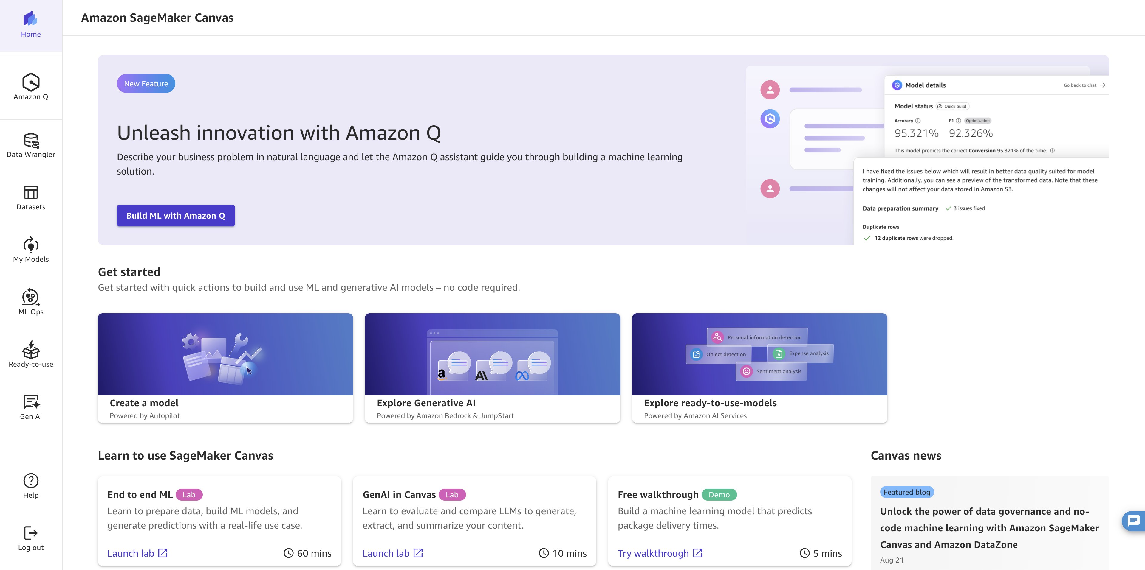
Figure 1: Amazon SageMaker Canvas workspace loading after opening it from the domain
Data Wrangler: ML data preparation
Amazon SageMaker Data Wrangler simplifies data preparation for machine learning workflows. With built-in transformations and an intuitive visual interface, Data Wrangler reduces the time traditionally spent on data preparation and analysis. For industries ranging from financial services to healthcare, this capability unlocks significant value so subject matter experts can directly prepare their data for analysis.
The integration with Snowflake reduces data movement challenges, so users can connect directly to their Snowflake data warehouses, transform the data within Canvas, and proceed straight to model building. This unified, no-code environment accelerates time-to-insight while maintaining data governance and security.
A. Data connection and initial setup
In this section, you connect Amazon SageMaker Canvas to a Snowflake data source.
- Navigate to Amazon SageMaker Canvas and choose Data Wrangler from the left navigation pane. Choose Import and prepare, then choose Tabular to work with structured datasets.
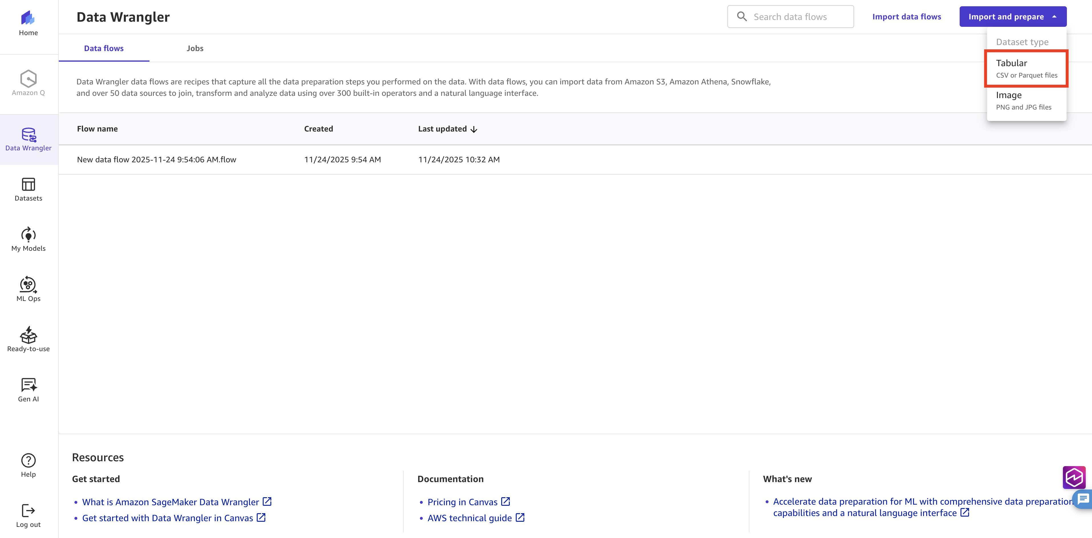
Figure 2: Amazon SageMaker Data Wrangler Import and prepare screen with Tabular selected
- Specify the source of your tabular dataset. From the data source menu, choose Snowflake as your connection type. Then choose Add Connection to establish the link between Amazon SageMaker Canvas and your Snowflake environment. With this integration, you can access your cloud data warehouse directly within Canvas. It avoids manual data exports and makes sure you are always working with the most current data in your Snowflake instance.
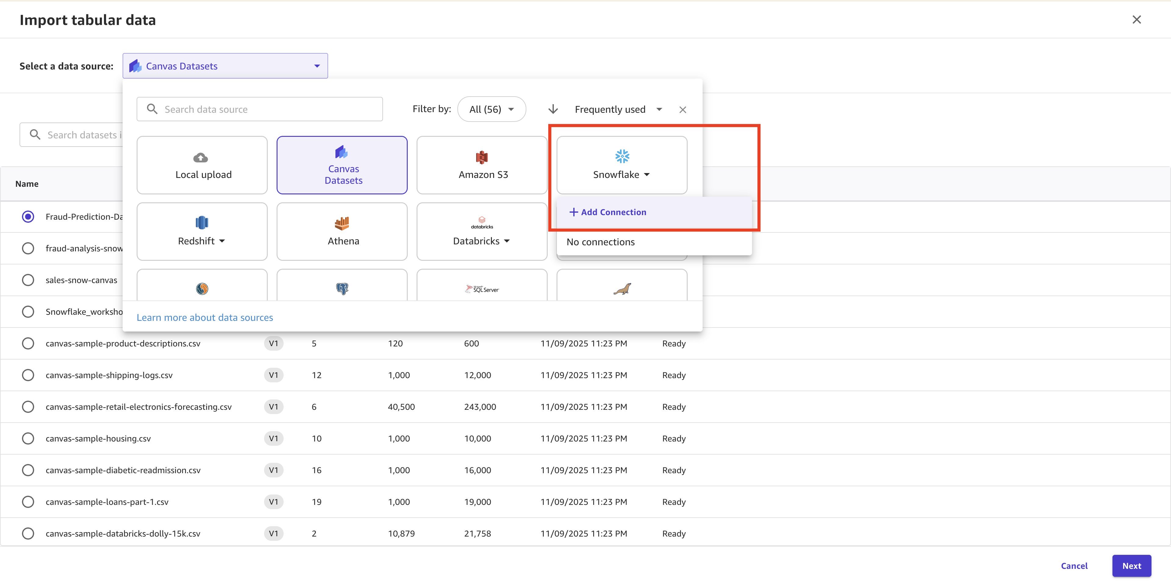
Figure 3: Selecting Snowflake as the data source and adding a connection in Data Wrangler
- In the Snowflake connection pop-up menu, provide the following:
- A connection name.
- The Account ID, set to your Snowflake organization value, plus a hyphen, plus the Snowflake account ID.
- The username for the Snowflake account you set up earlier.
- The password that you set previously.
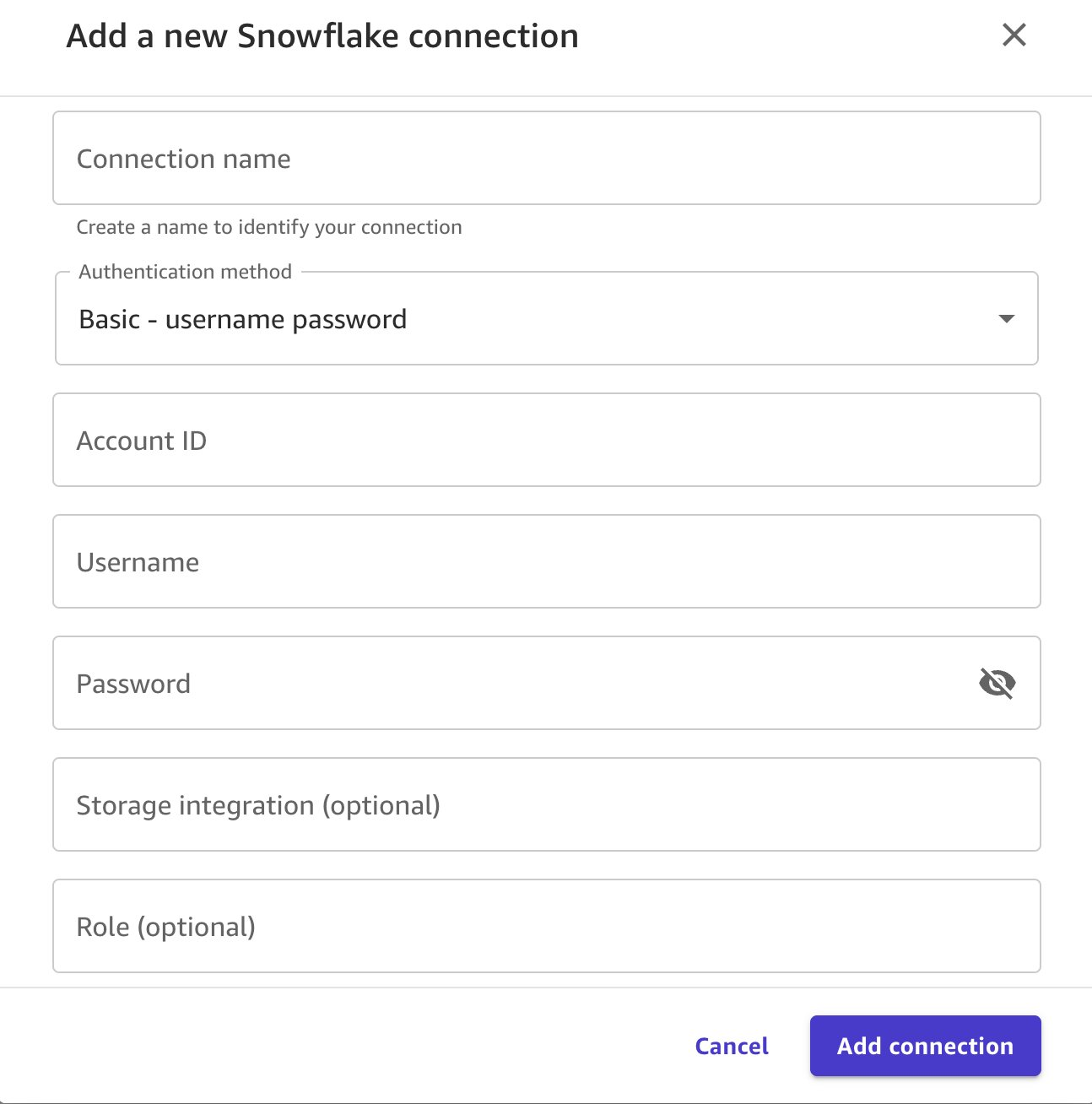
Figure 4: Snowflake connection dialog with connection name, account ID, username, and password fields
- After the connection is established, you will create card-level outlier thresholds to identify unusual spending patterns for each credit card and category combination. This helps the model detect when a transaction amount significantly deviates from a cardholder’s typical behavior. Copy the SQL query to prepare the fraud detection dataset.
- Run the query:
- Choose Edit in SQL in the top right corner to open the SQL editor.
- Paste the SQL query into the editor.
- Choose Run SQL to run and preview results.
- Choose Import to bring the dataset into your Canvas workspace.
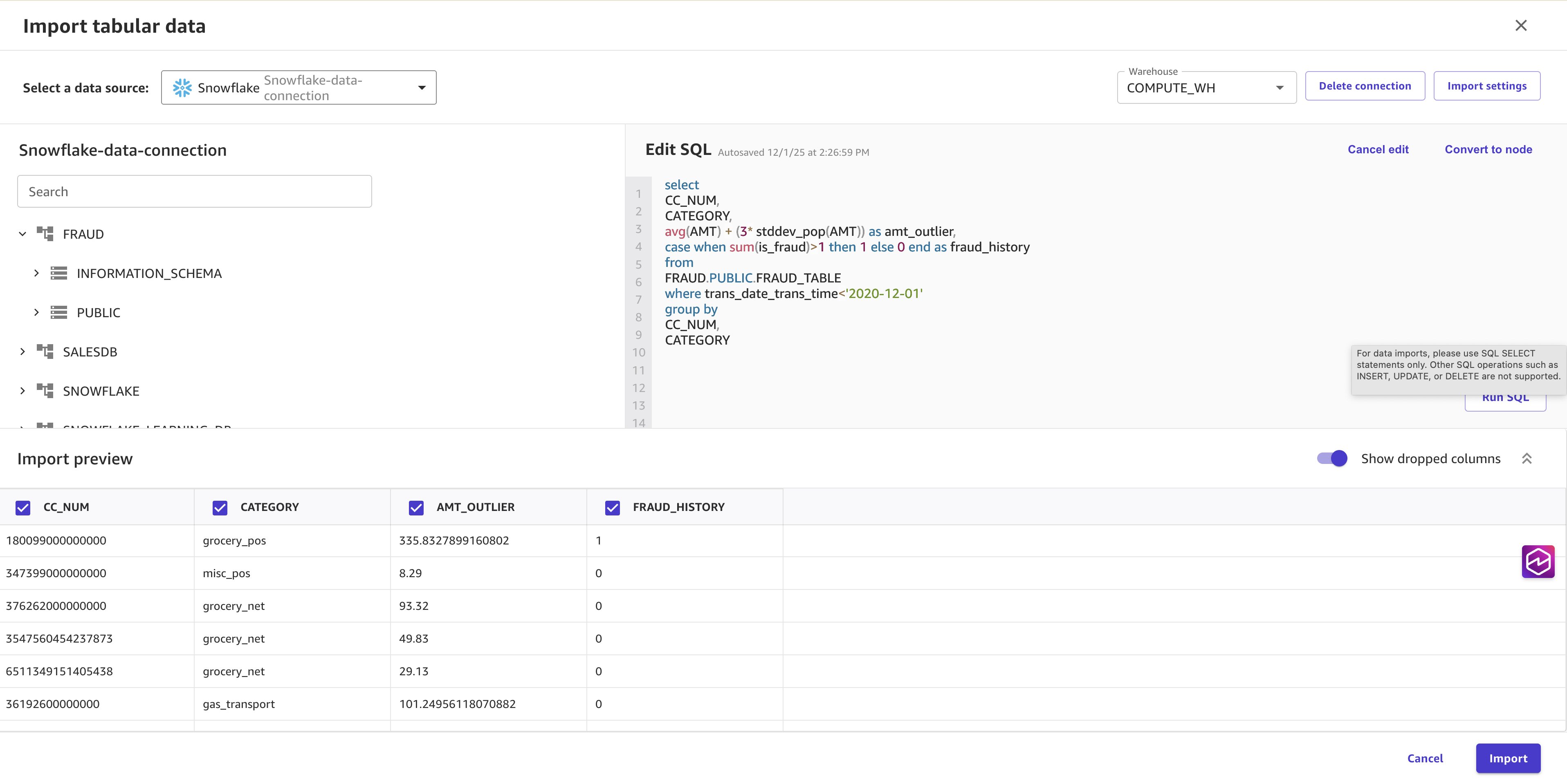
Figure 5: SQL editor in Data Wrangler showing the outlier-threshold query results ready to import
B. Data enrichment
In the following steps, you will enrich the dataset with transaction-level features and merchant-specific fraud indicators.
- Choose Data flow to add more data. In the top right corner, choose Add Data, and then choose Tabular.
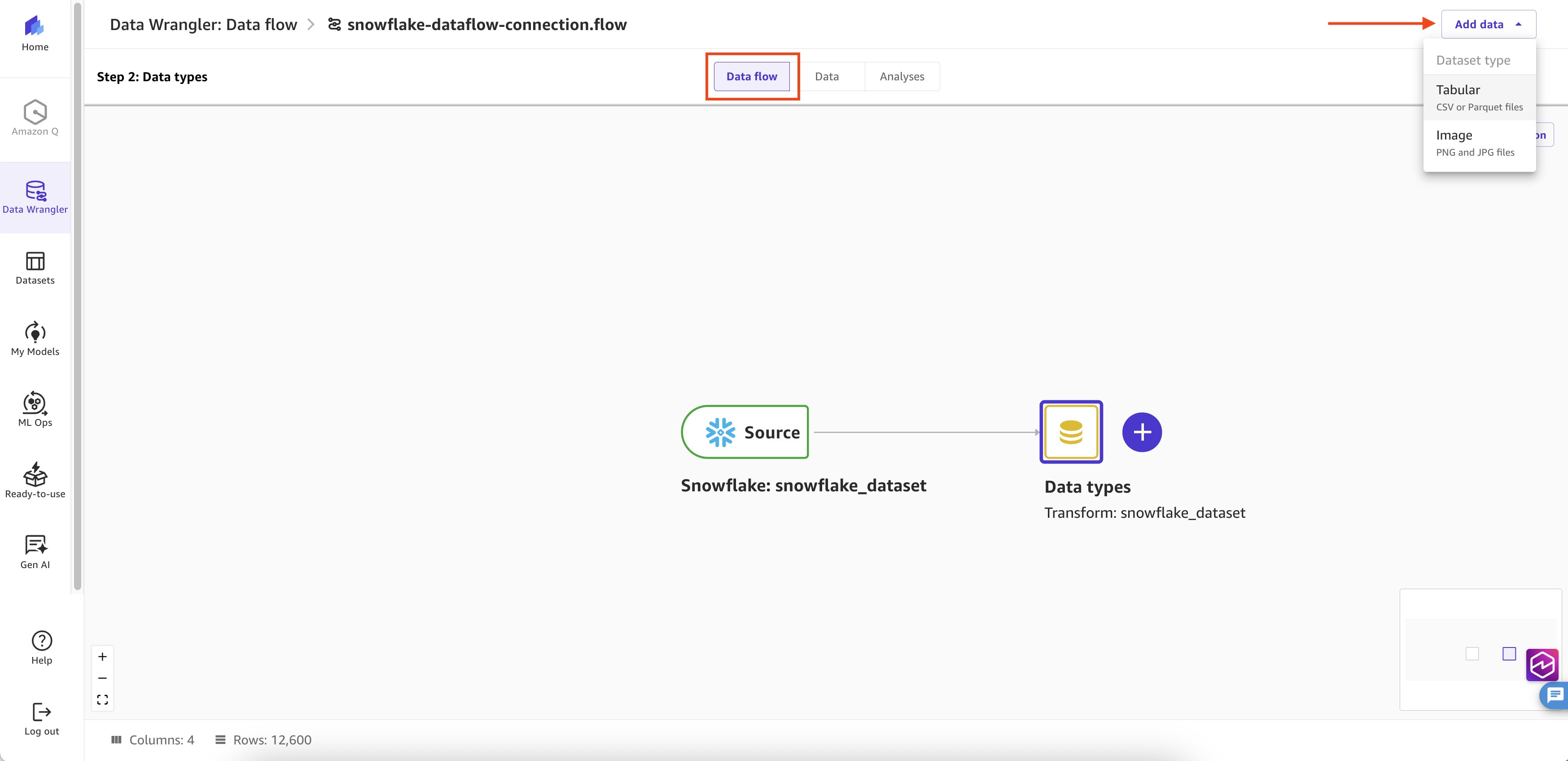
Figure 6: Data flow canvas with the Add Data and Tabular options for adding a second source
- Choose the data source as Snowflake and the existing connection you created before.
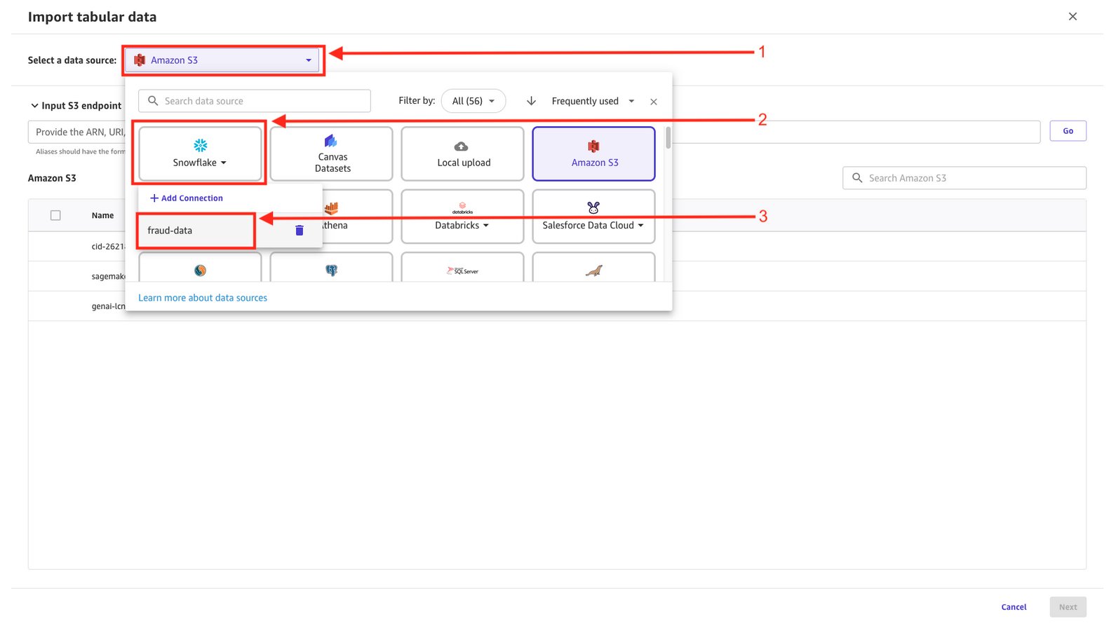
Figure 7: Selecting the existing Snowflake connection for the second data source
- In the Edit SQL window, paste the SQL query. This query provides temporal patterns (hour of day, day of week), demographic information (age categories), and merchant-level outlier thresholds, all critical signals for fraud detection. Choose Run SQL, then choose Import.
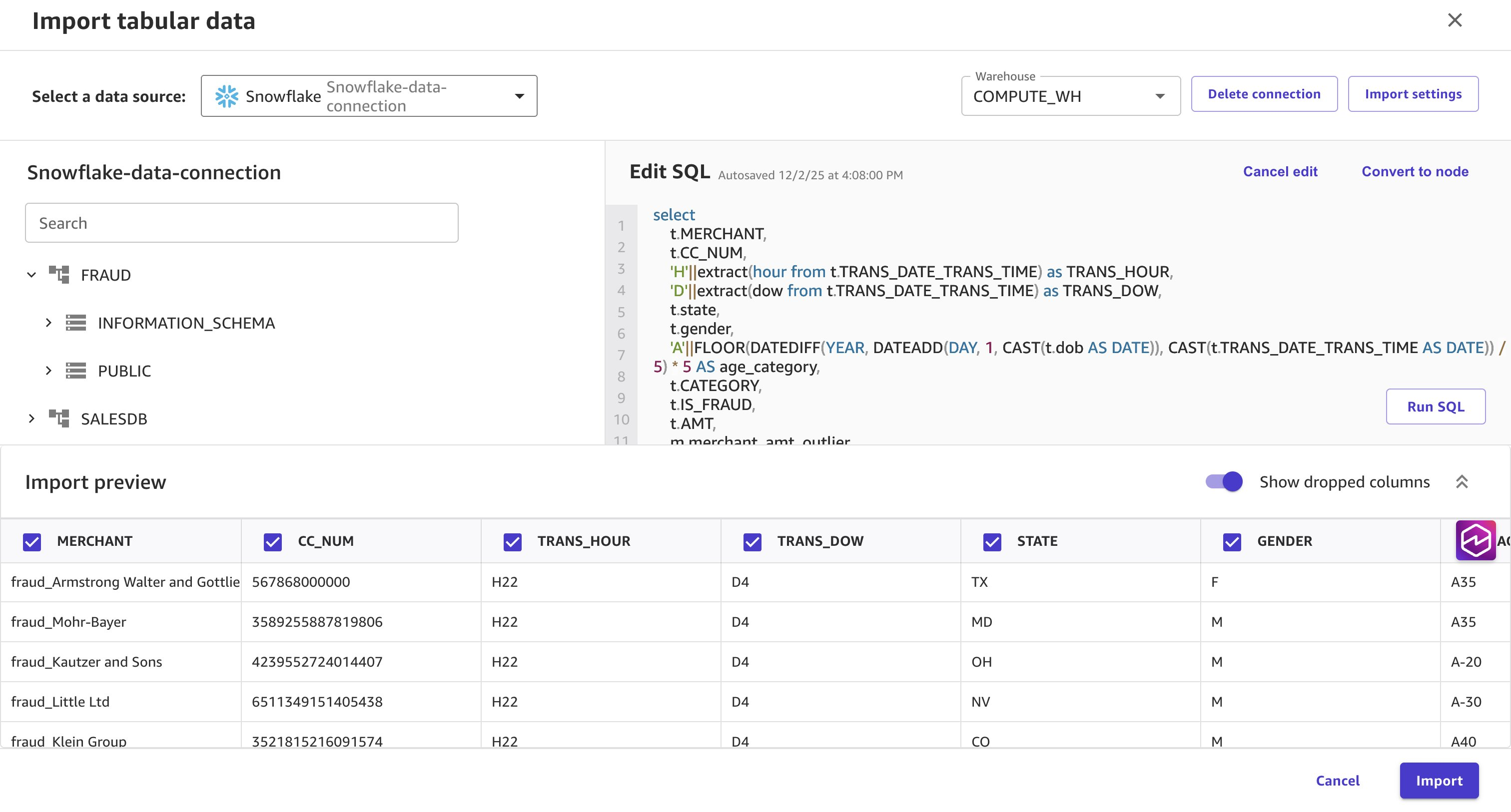
Figure 8: Data Wrangler preview of the enrichment query with temporal, demographic, and merchant features
C. Data transformation
In this section, you will join the data together.
- On the Data flow screen, you see the two data sources imported from Snowflake. Choose the first data type and choose the plus icon next to it. Choose Combine data, then Join. When the right panel opens, choose the second data type from the data flow to join.
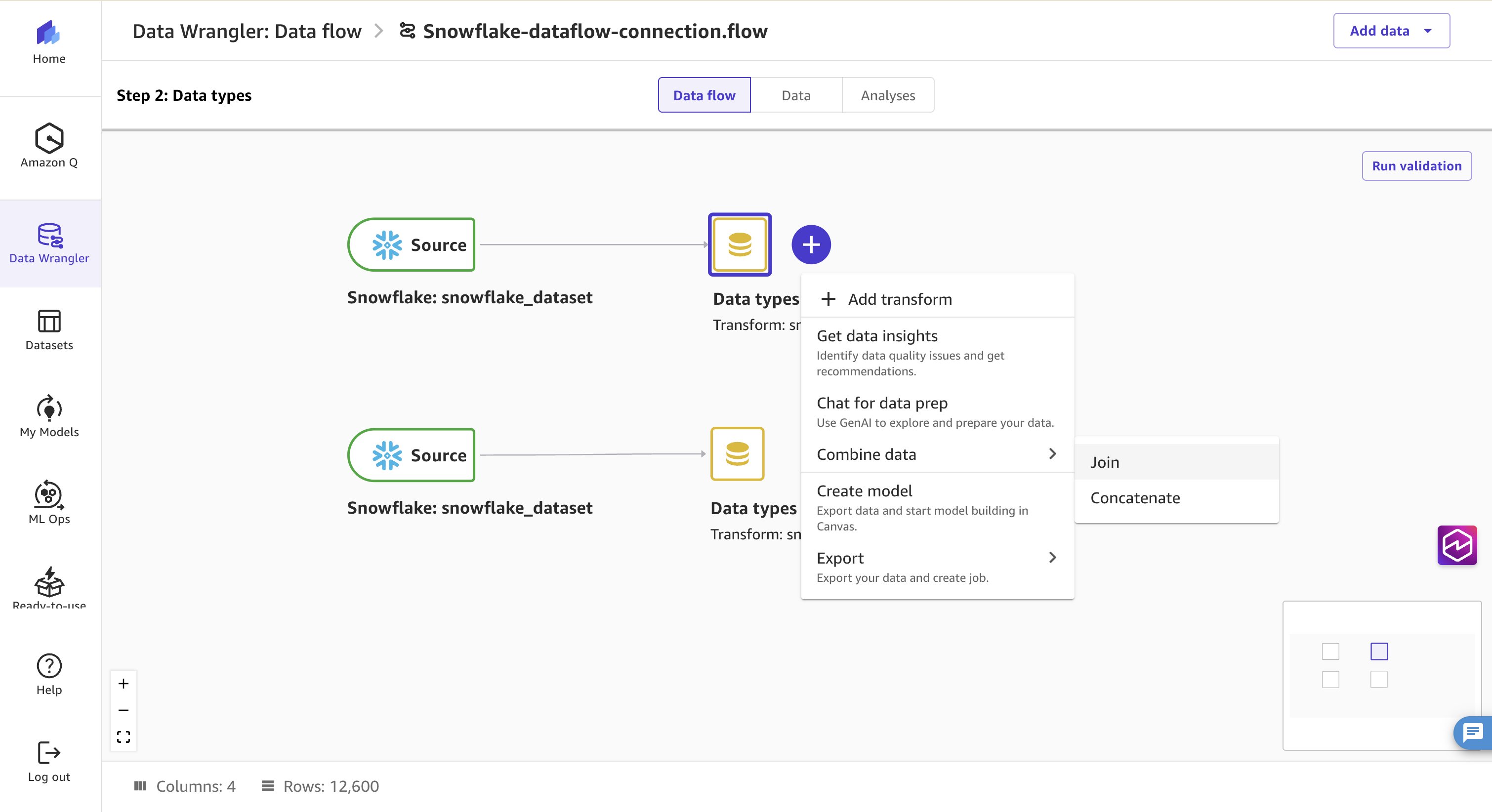
Figure 9: Data flow showing the Combine data and Join options between the two Snowflake sources
- Choose Left outer join for the Join type. Add a Join key and choose Category as the left and right join key.
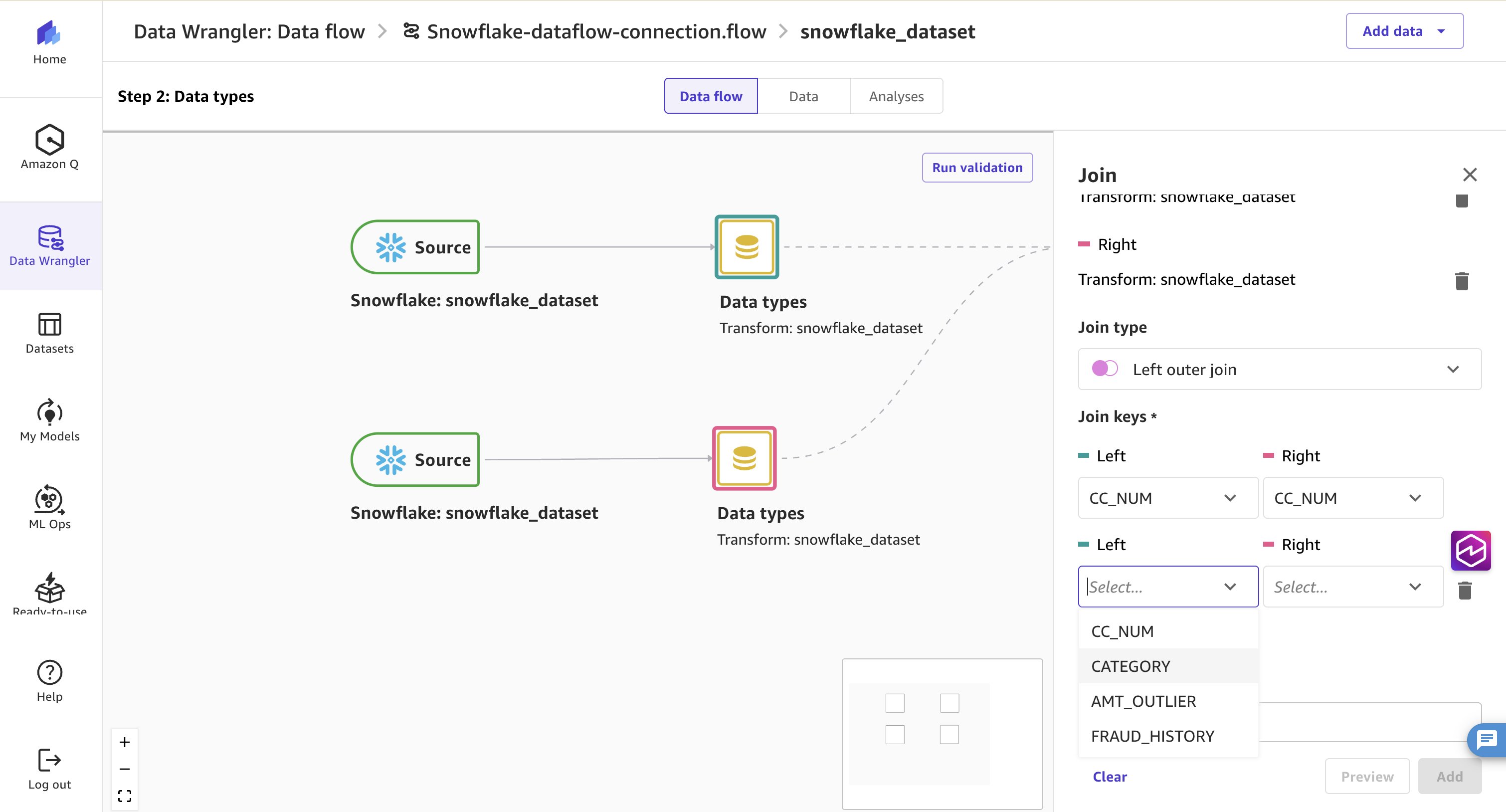
Figure 10: Join configuration with Left outer join type and Category as the join key
- Choose Preview to view the joined data. Choose Add to proceed.
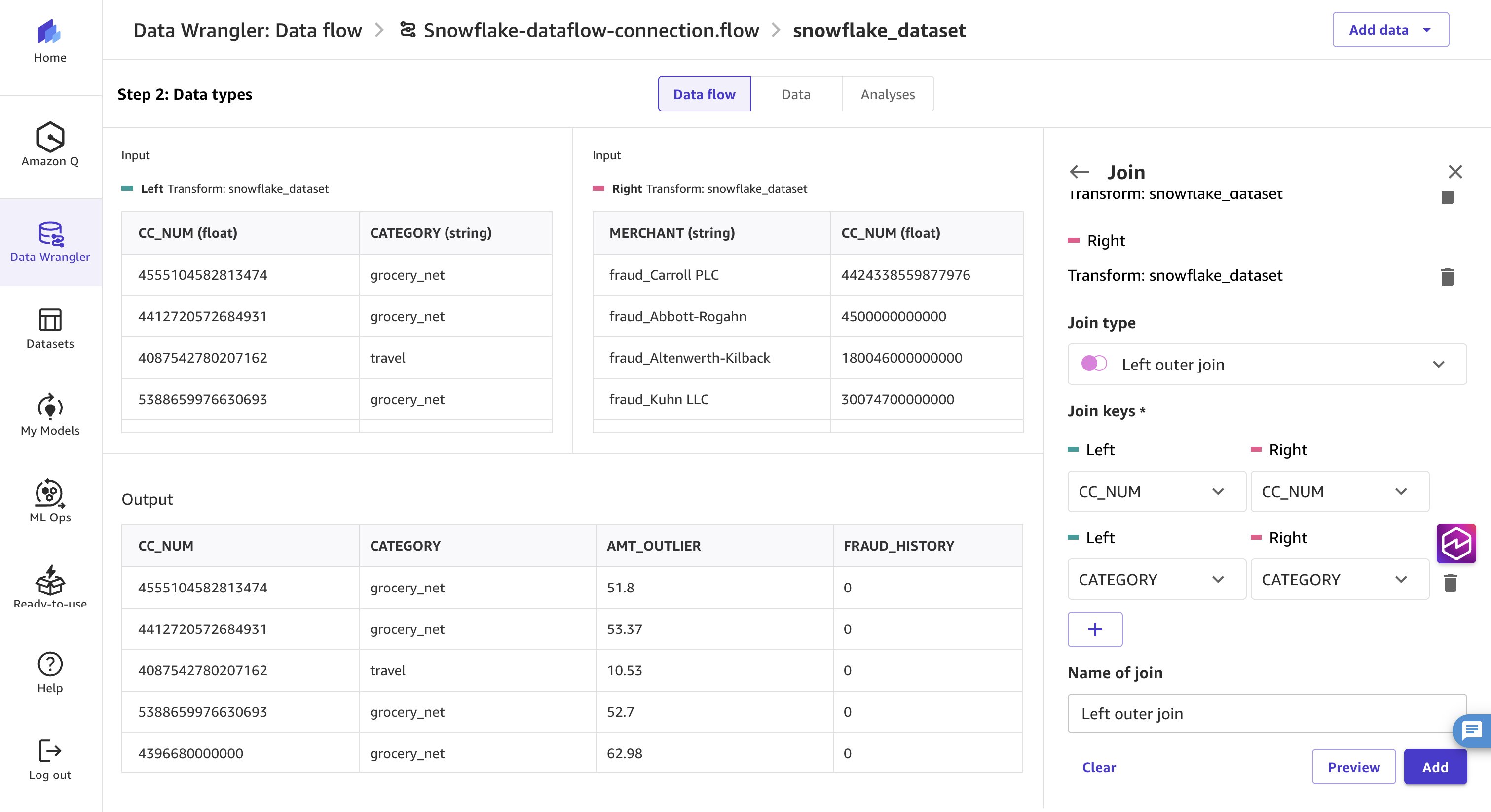
Figure 11: Preview of the joined dataset before adding it to the data flow
Next, you will create outlier features and remove sensitive columns.
- Return to the Data flow screen, choose the join, choose the plus sign (+) next to it, and then choose Add transform.
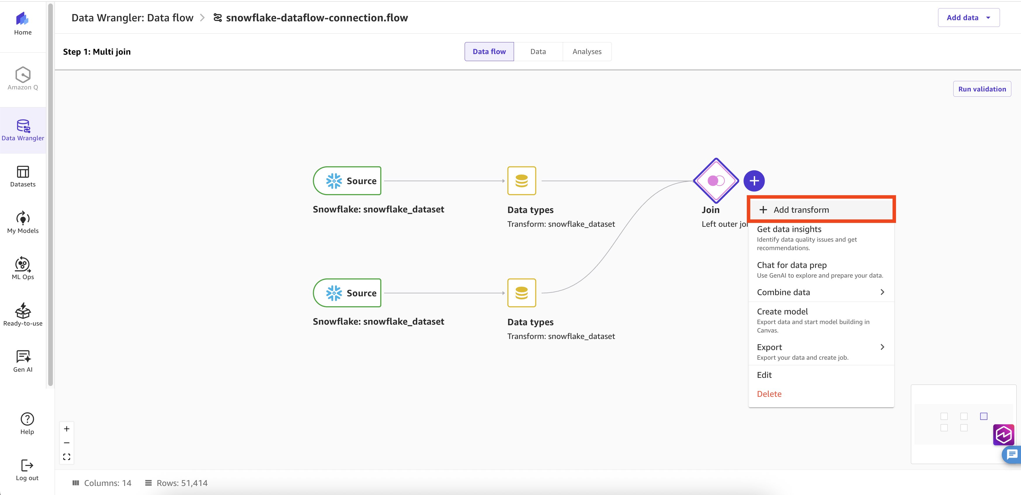
Figure 12: Adding a transform to the join node in the data flow
- After the interface opens, choose Add transform in the right-hand panel, and then choose Custom Formula.
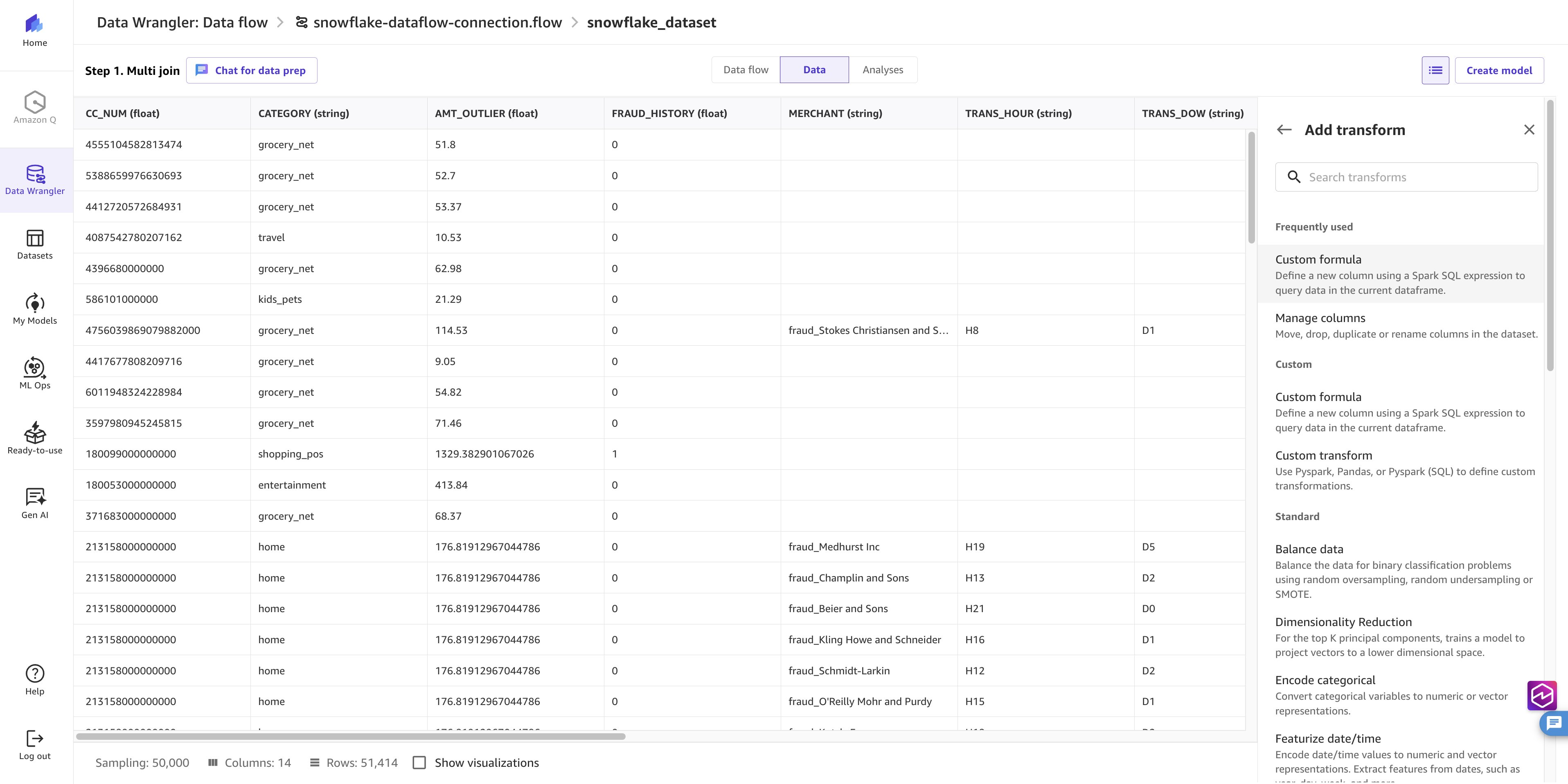
Figure 13: Choosing Custom Formula in the Add transform panel
- This option gives you the flexibility to add columns using a Spark SQL expression. Copy and paste the following Formula on the Home tab. Enter the output column as
CC_FLAGand choose Add.
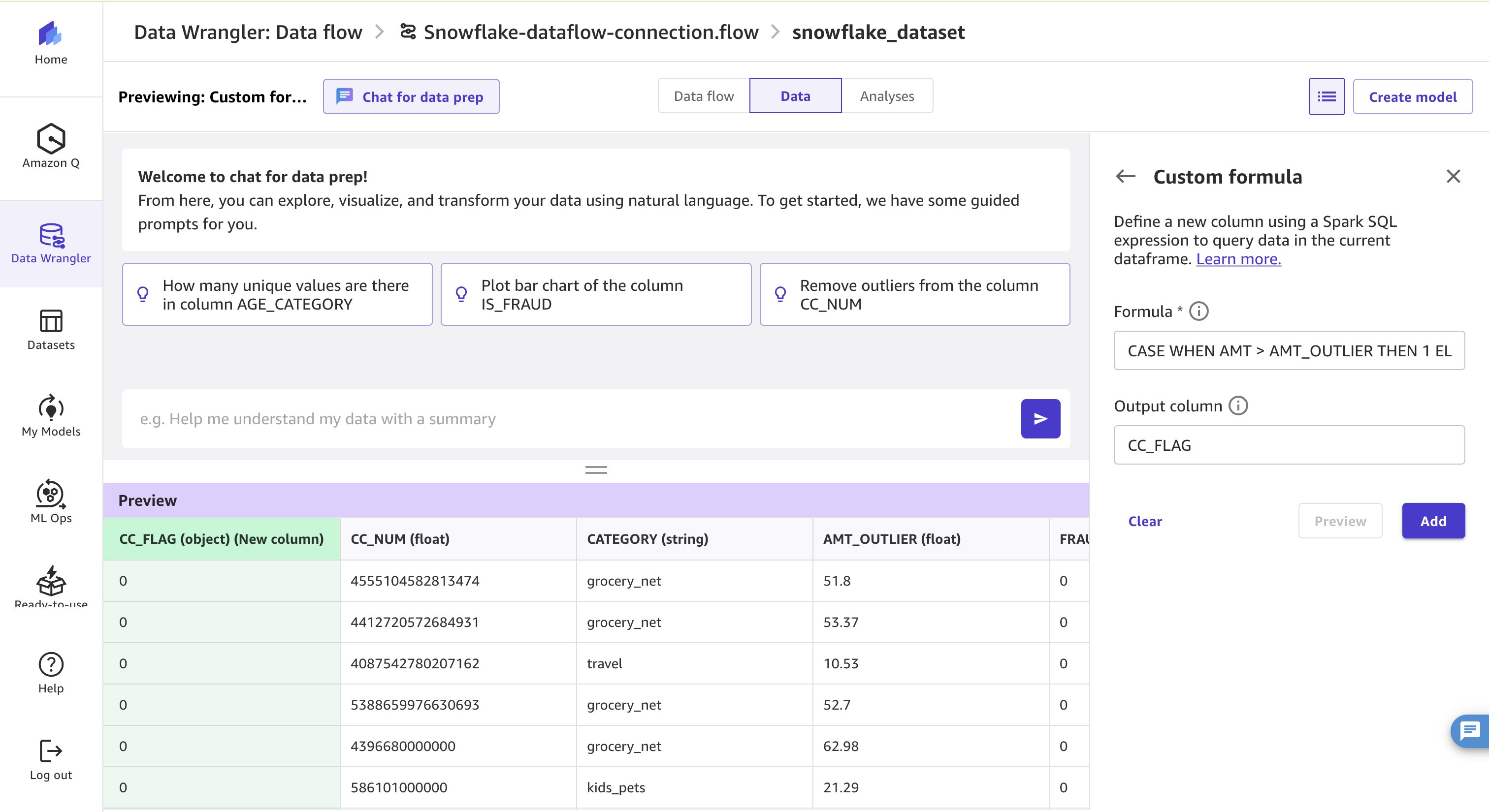
Figure 14: Custom formula creating the CC_FLAG column from the card outlier threshold
- To add another column, repeat the same steps to enter a custom formula, then copy and paste this query and name the output column as
MERCHANT_AMT_FLAG.
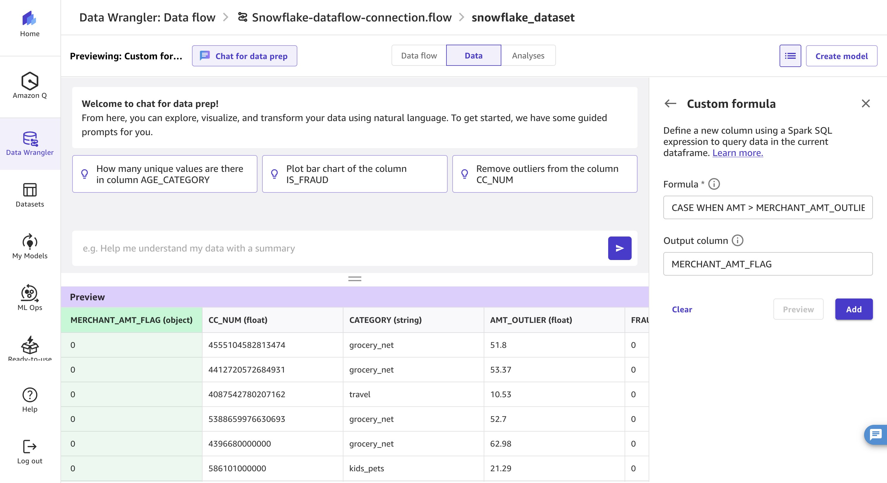
Figure 15: Custom formula creating the MERCHANT_AMT_FLAG column from the merchant outlier threshold
- To make sure the model remains free of sensitive information such as card numbers, merchant names, and outlier amounts tied to cards or merchants, remove these columns using built-in transformation.
- Select Add transform and choose Manage Columns
- Select the Transform type to Drop column
- Select the columns you want to remove from your dataset
- Choose Add to apply the transformation.
CC_NUM.AMT_OUTLIER.MERCHANT.MERCHANT_AMT_OUTLIER.
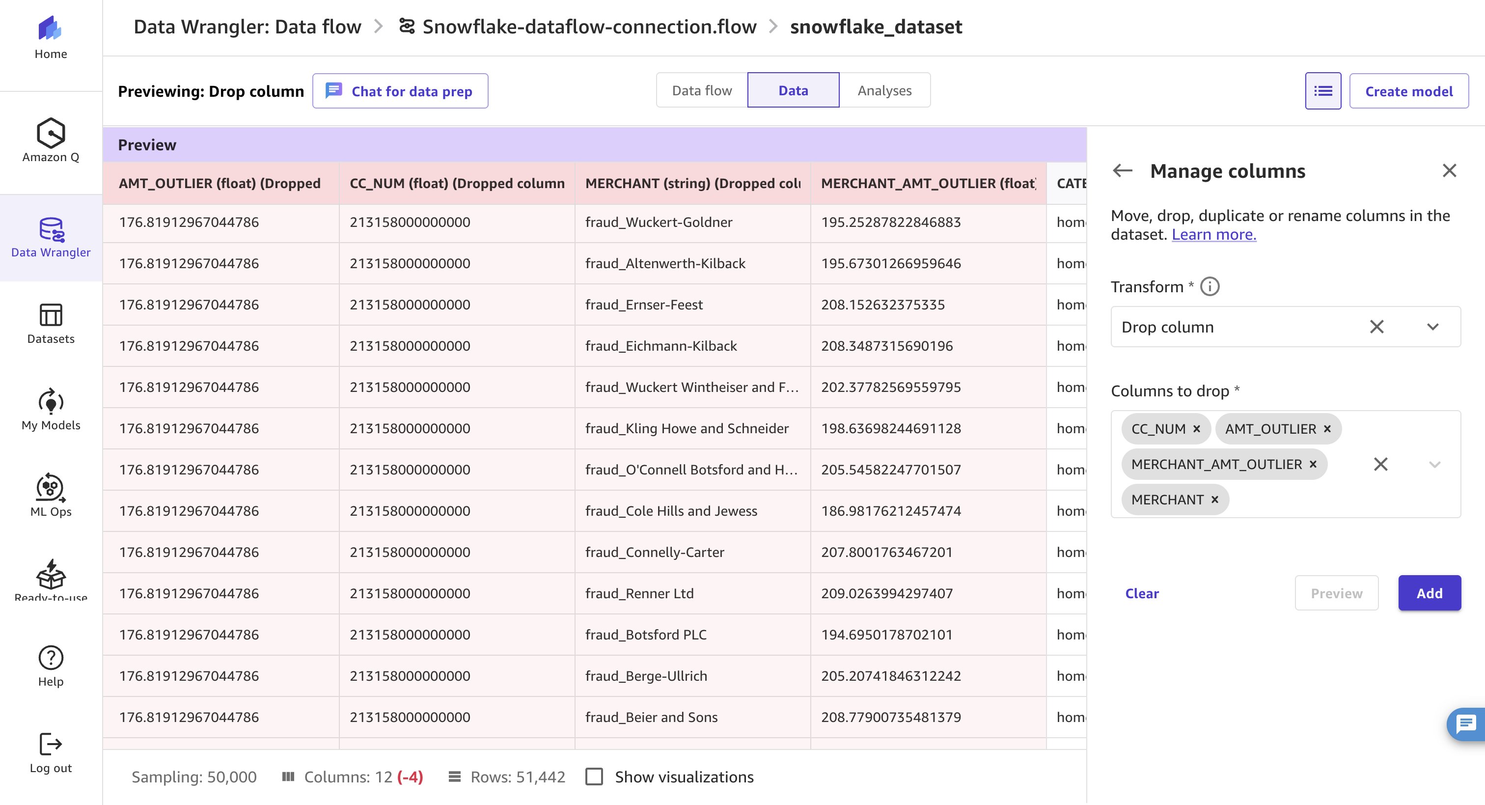
Figure 16: Manage Columns transform dropping sensitive columns from the dataset
D. Quality analysis and model export
With data preparation complete, you will run a quality analysis report to get insights into the data. The insights report identifies common data issues, such as target leakage or class imbalance, helping users address them early in the workflow.
- To initiate the analysis, choose the Analyses tab. In the right-hand panel, choose Data Quality and Insights Report from the Analysis type list.
- Choose
IS_FRAUDas the target column. This tells Canvas which variable you want to predict. Then choose the Classification option under Problem type. The Data size should remain as Sampled Dataset. Finally, choose Create to launch the analysis.
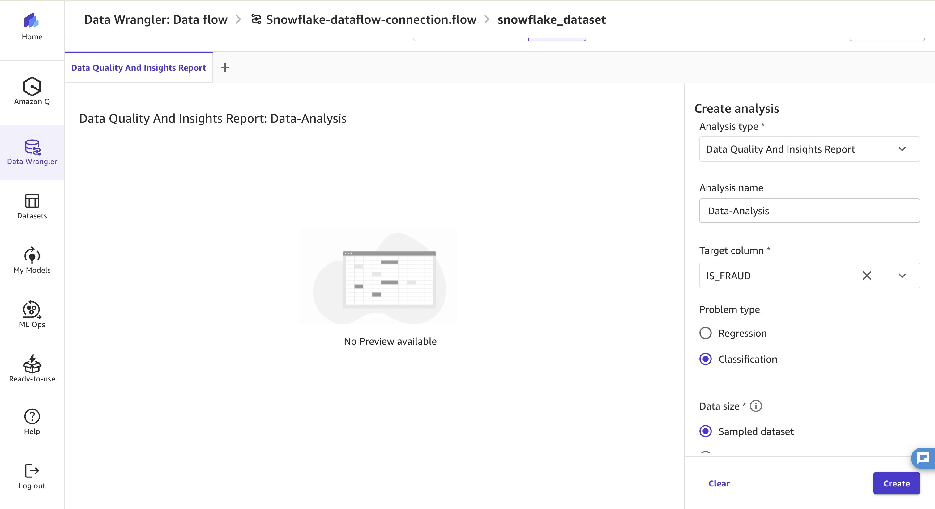
Figure 17: Data Quality and Insights Report configuration with IS_FRAUD target and Classification problem type
- Within a few minutes, a detailed analysis report will be created which includes a quick summary of the data, feature summary, duplicate rows, anomalous samples and much more. In the Quick model section, review the accuracy metrics in the training and validation datasets. A confusion matrix follows the accuracy statistics. The idea is to use this report after any data engineering to observe how it impacts model quality.
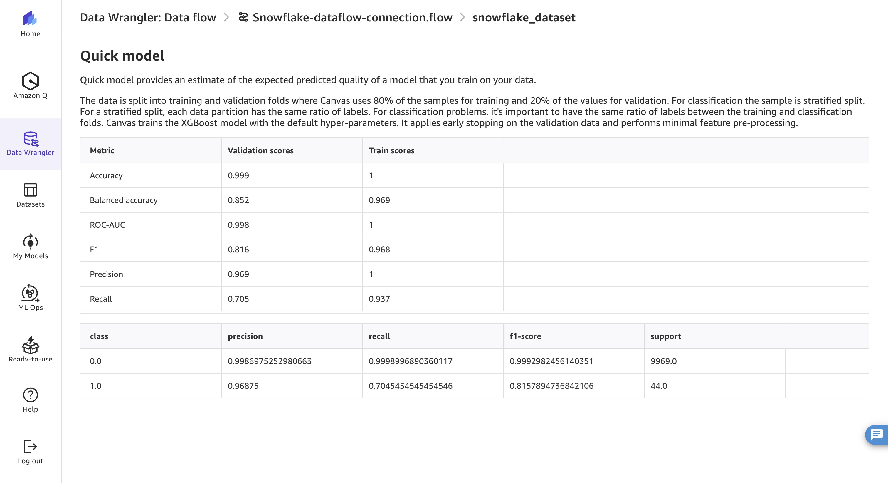
Figure 18: Data quality and insights report with Quick model accuracy metrics and confusion matrix
- The feature summary section shows feature importance. In practice, if there are features with low prediction power, you might choose to drop those features.
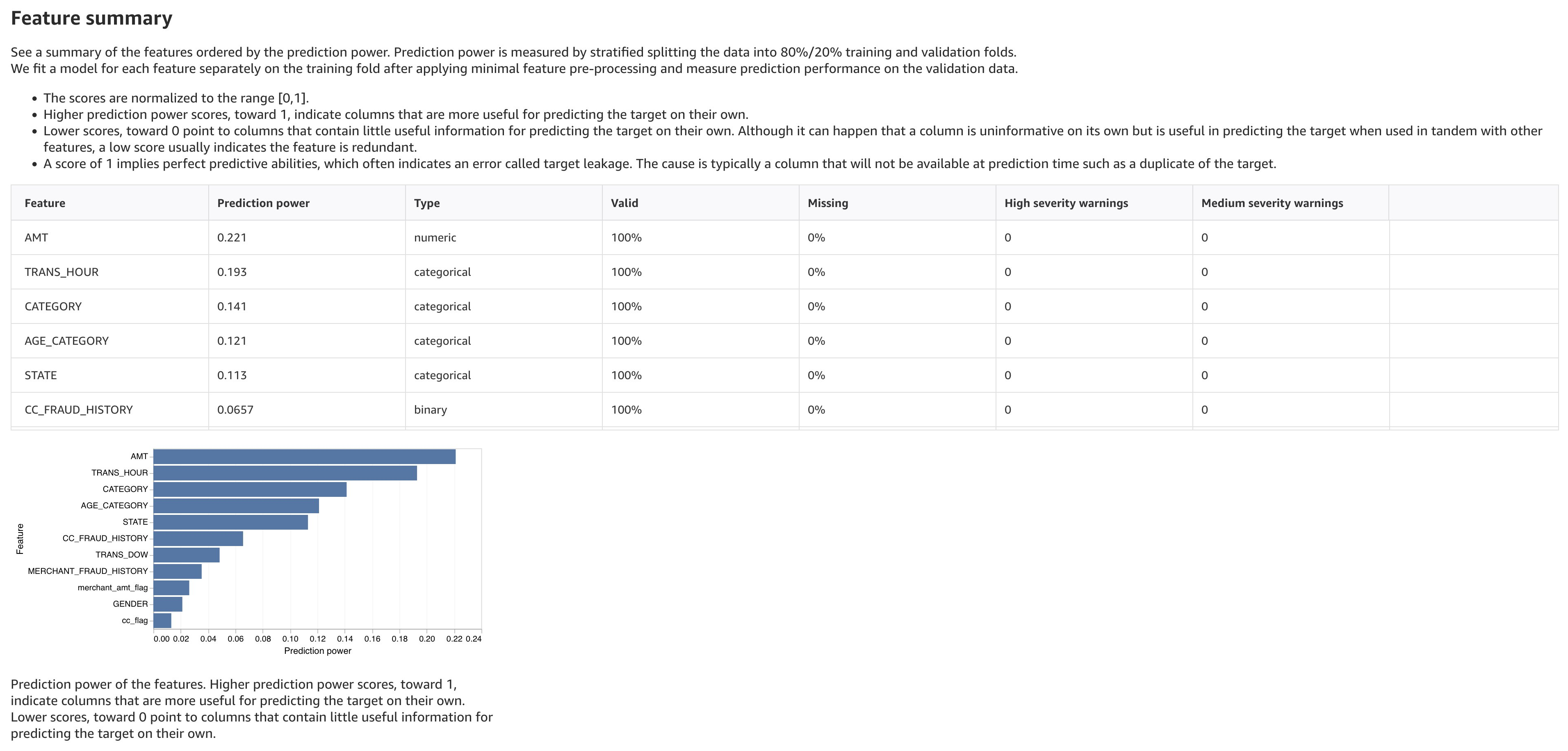
Figure 19: Feature summary section of the insights report showing feature importance
Export to model building
You’ve now combined two data sources, engineered new features, removed unnecessary ones, and previewed your model’s potential accuracy by running the analysis. With data preparation complete, it’s time to build your predictive model.
- To begin, return to the Data flow tab, choose the plus sign (+) next to your final transform, and then choose Create model.
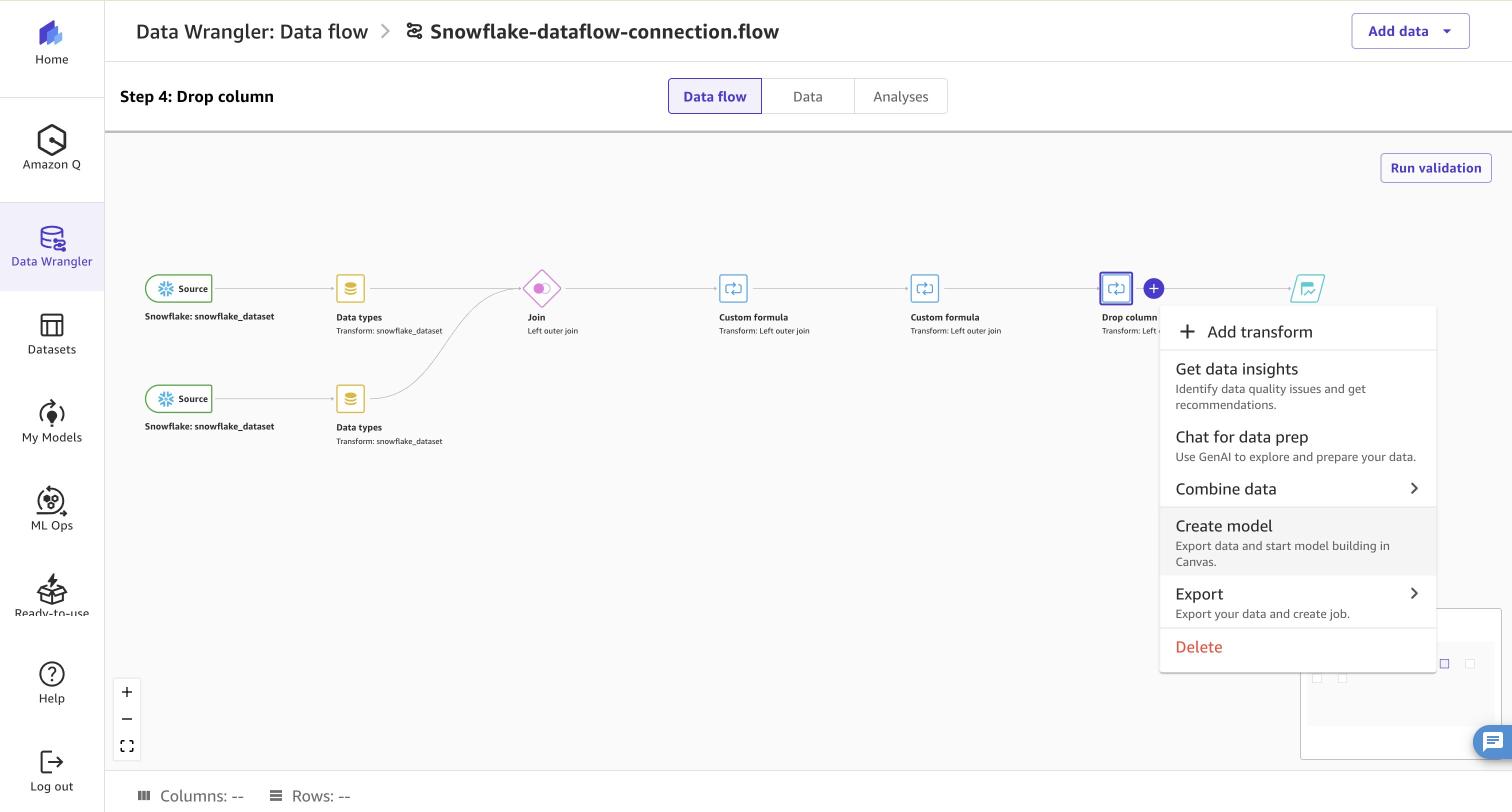
Figure 20: Creating a model from the final transform node in the data flow
- Choose a descriptive name under Model name, and then choose Export and create model. The export process may take a few minutes as Canvas processes your entire dataset in real time.
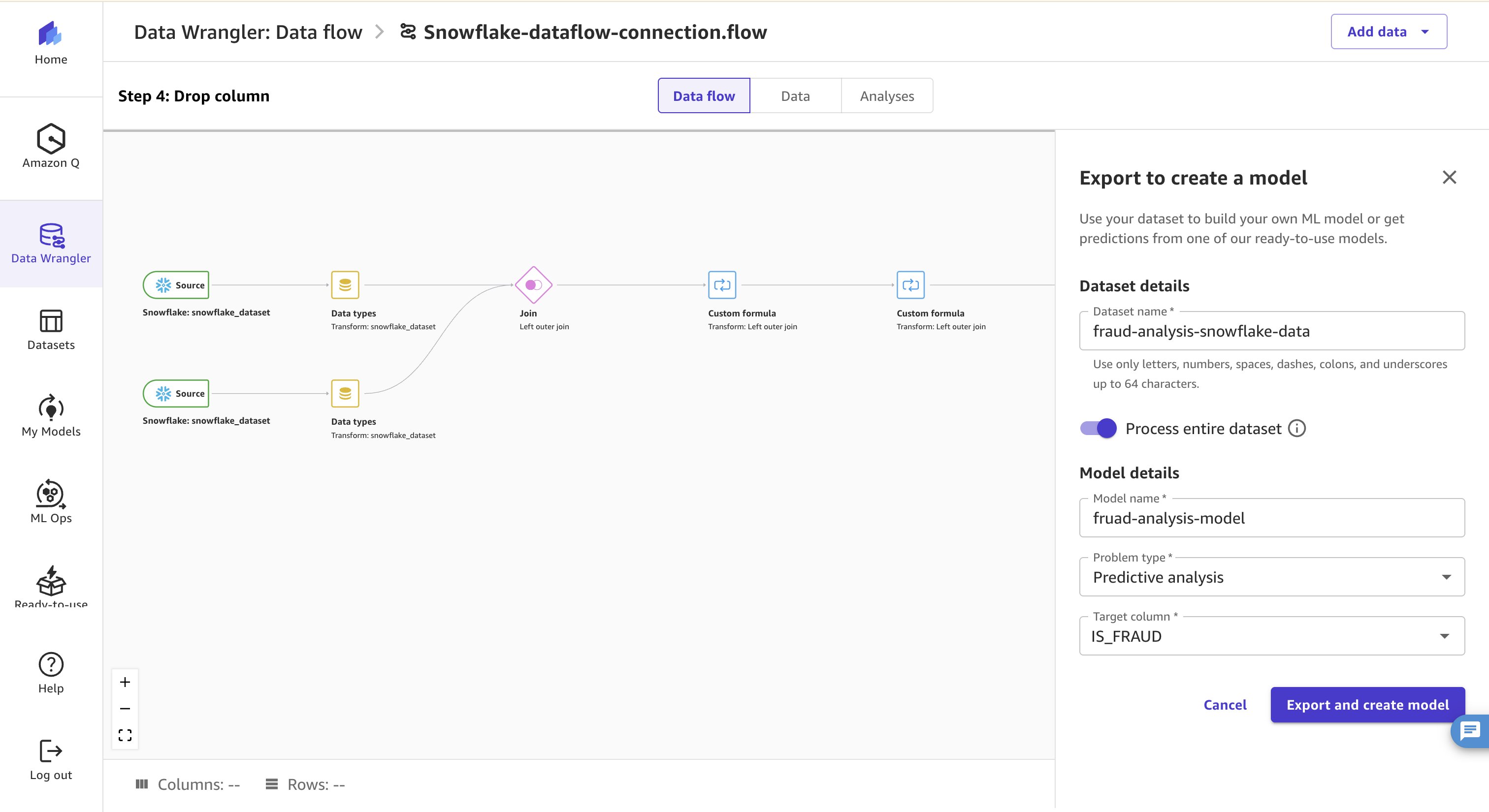
Figure 21: Model name entry and the Export and create model action in Canvas
After a few minutes, the Build screen opens up.
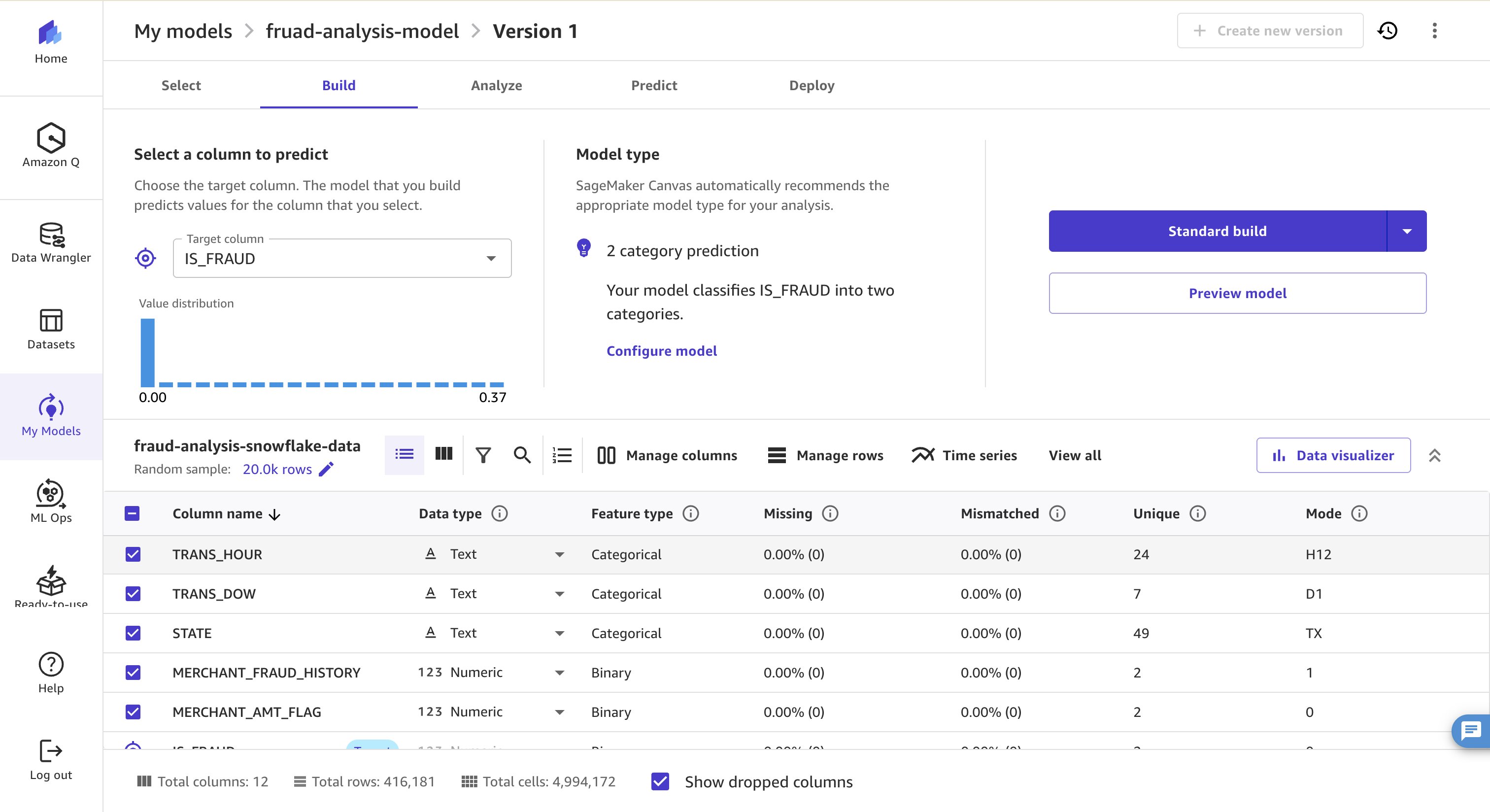
Figure 22: Canvas Build screen after exporting the prepared dataset
- Choose
IS_FRAUDas the Target Column. - Choose Configure model under Model type. Select 2-category model as model type.
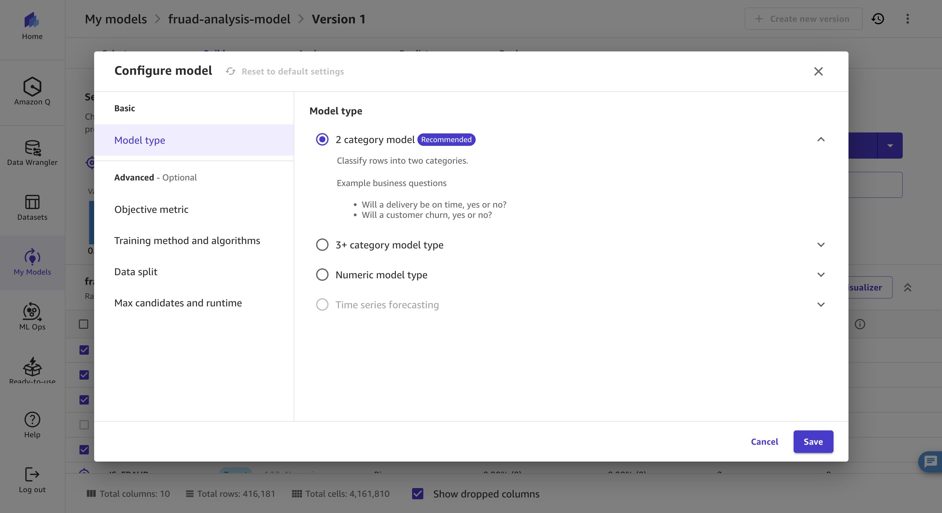
Figure 23: Configuring a 2-category model type in Canvas
- Next, select Ensemble as the training method with XGBoost as the algorithm, a strategic choice that balances accuracy with efficiency.
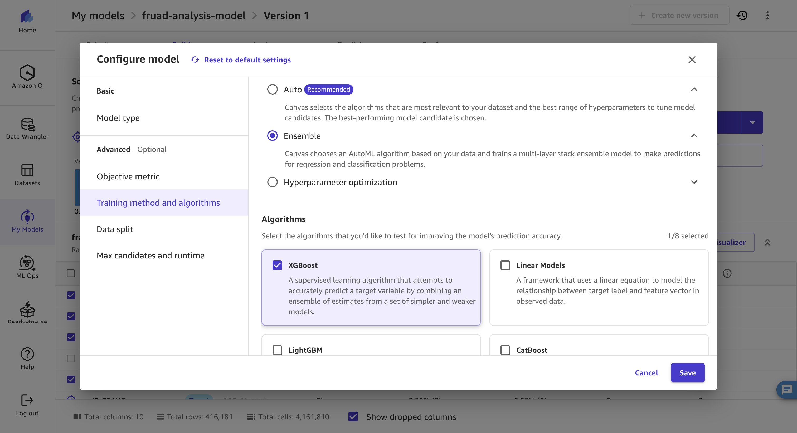
Figure 24: Selecting the Ensemble training method with the XGBoost algorithm
- Deselect the FRAUD_HISTORY and MERCHANT_FRAUD_HISTORY columns, then choose Standard build to start training. The model takes approximately 15–30 minutes to complete.
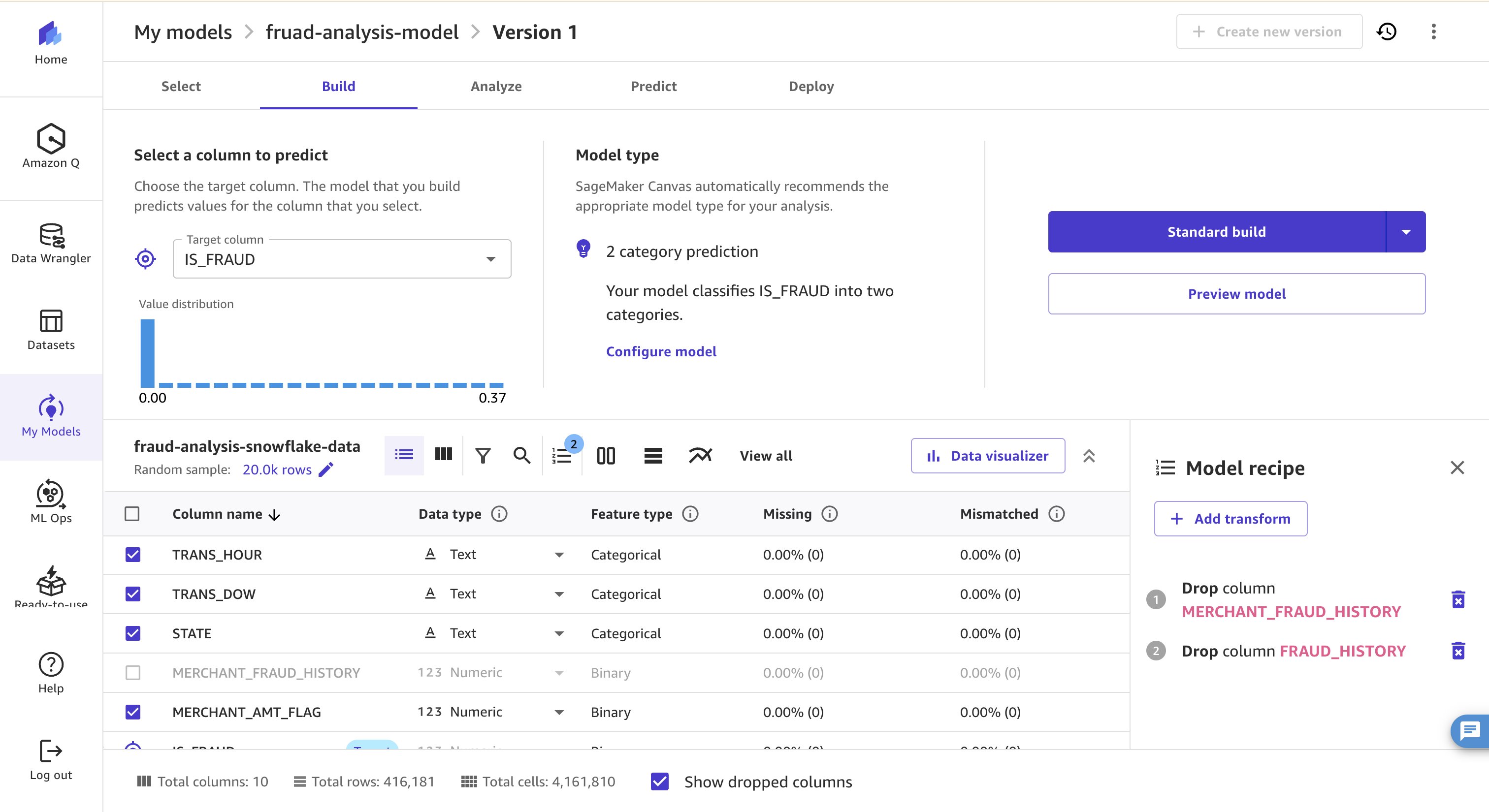
Figure 25: Deselecting history columns and starting a Standard build
- With the model training complete, navigate to the Analyze tab to review the results. Here, you can examine which features had the most impact on predictions and explore the scatterplot and charts to understand relationships between data values and fraud classification.
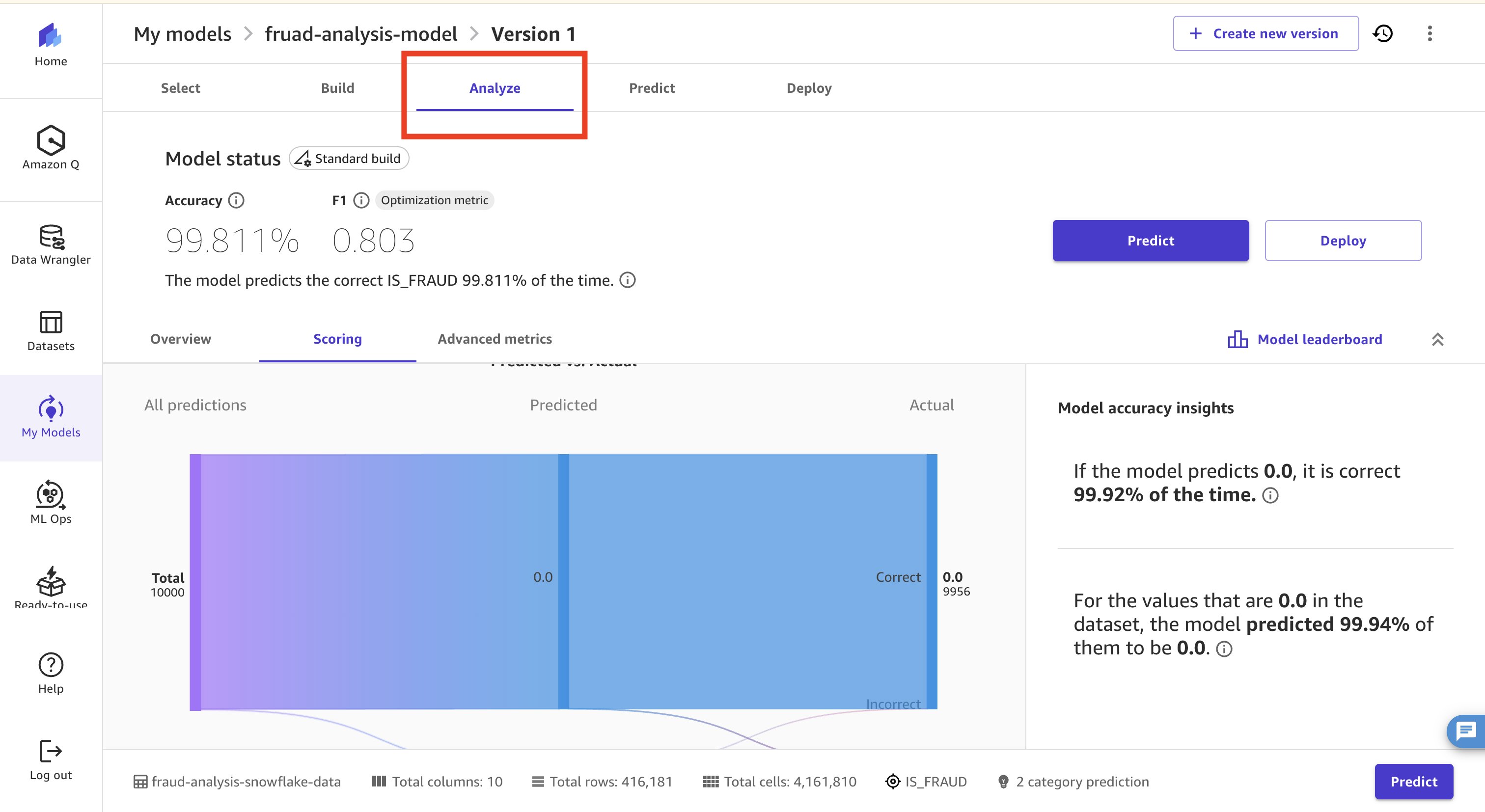
Figure 26: Canvas Analyze tab showing feature impact and fraud classification charts
- Choose Advanced Metrics to further understand model performance.
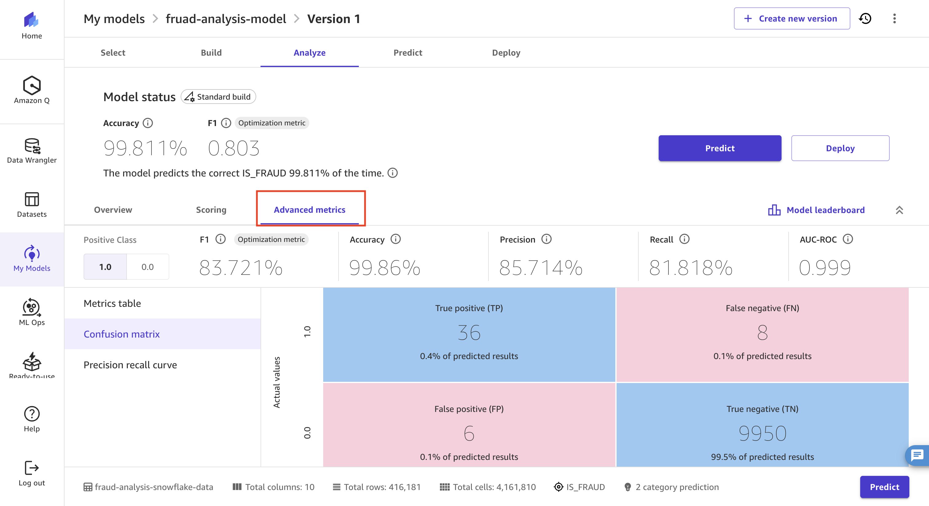
Figure 27: Advanced Metrics view of the trained fraud detection model
- Next, use the trained model to make predictions on an unseen dataset. Download the sample prediction CSV file. Navigate to the Predict tab. Choose Manual, and then choose Create Dataset.
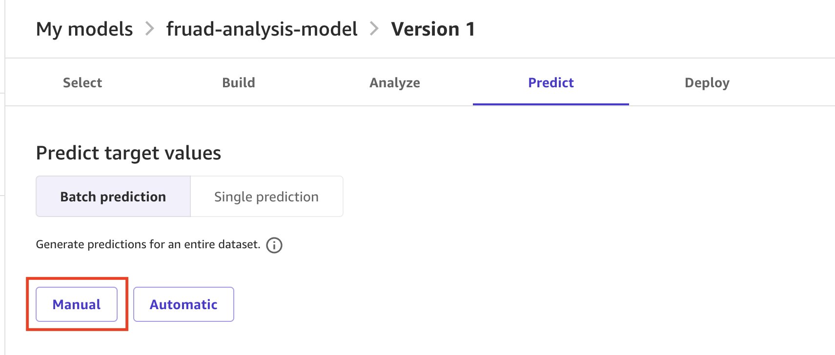
Figure 28: Predict tab with Manual dataset creation for generating predictions
- Upload the dataset, choose Preview dataset, and then choose Create dataset. After the dataset loads, choose the dataset and choose Generate Predictions. The model takes a few minutes to make the predictions. Wait until the status of the job changes to Ready.
- To analyze the results visually using Amazon Quick Sight, you must first verify the following prerequisites (detailed here):
- Verify AWS Region alignment: Your Quick Sight account must be set up in the same AWS Region as your Amazon SageMaker Canvas domain.
- Add Amazon Quick Sight permissions to your Amazon SageMaker execution role: The AWS Identity and Access Management (IAM) execution role attached to your Amazon SageMaker domain needs additional permissions to send predictions to Amazon Quick Sight. Navigate to the IAM console, find the execution role associated with your Amazon SageMaker domain (created during setting up Amazon SageMaker domain at the very beginning), and add the required inline policy as described here.
- Grant Quick Sight access to the Amazon SageMaker S3 bucket: Navigate to Quick Sight, go to Manage Accounts, then choose AWS Resources from the left-hand navigation pane. Make sure Amazon Simple Storage Service (Amazon S3) is selected and choose the appropriate S3 bucket that has the predictions generated by Amazon SageMaker Canvas, named sagemaker-{region}-{account_id}.
- Add Quick Sight users: Make sure the users you want to share predictions with have been added to your Quick Sight account with an Author or Admin role. Go to Manage Quick Sight and navigate to Manage users to invite new users or verify existing ones. For details, see Managing user access. You will enter their usernames when sending predictions.
- Next, select the Job name and choose Send to Amazon Quick Sight.
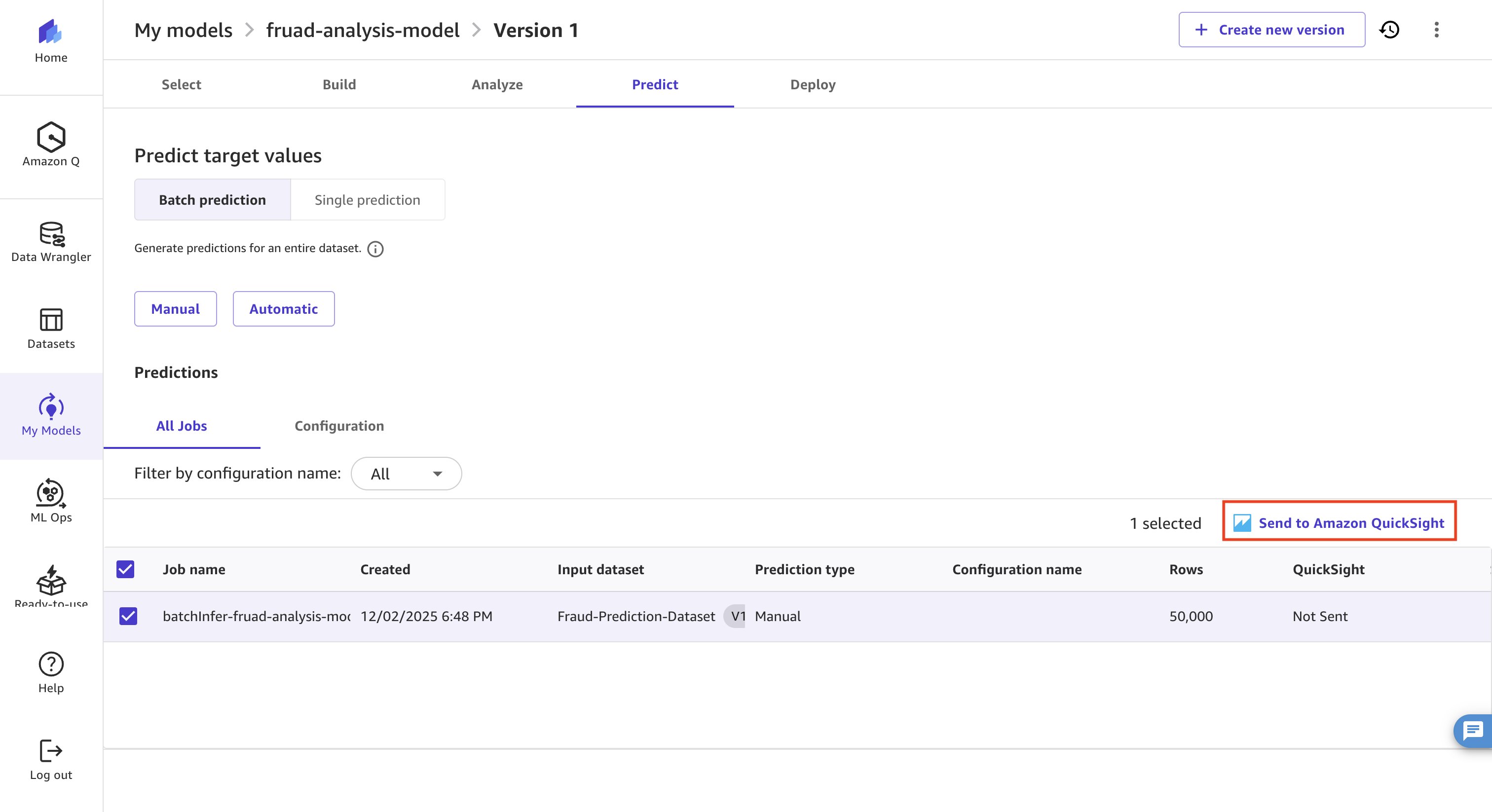
Figure 29: Selecting the prediction job and sending results to Amazon Quick Sight
- In the new window, add the users who were previously granted Amazon Quick Sight permissions as viewers of the dashboard, and then choose Send.
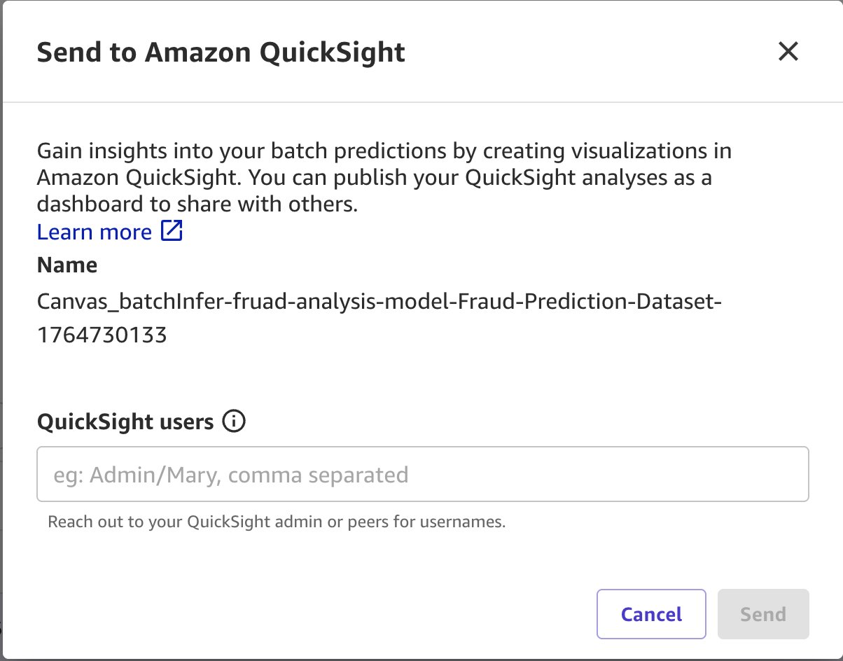
Figure 30: Adding dashboard viewers before sending predictions to Amazon Quick Sight
Conclusion
Part 2 covered the complete data preparation and model building workflow in Amazon SageMaker Canvas from connecting to Snowflake data sources and engineering features using Data Wrangler’s visual transformations, to joining multiple data sources, analyzing data quality, and training a fraud detection model all without requiring machine learning programming expertise. With the trained model now generating predictions on unseen data, the foundation is set for Part 3, where those ML-driven insights are brought to life through interactive dashboards in Amazon Quick Sight.
References
- Part 1 – Build a no-code ML workflow with Snowflake, Amazon SageMaker Canvas and Amazon Quick – Part 1: Setting up your Snowflake environment
- Part 3 – Build a no-code ML workflow with Snowflake, Amazon SageMaker Canvas and Amazon Quick – Part 3: Visualizing insights with Amazon Quick Sight