Artificial Intelligence
Prepare data for predicting credit risk using Amazon SageMaker Data Wrangler and Amazon SageMaker Clarify
For data scientists and machine learning (ML) developers, data preparation is one of the most challenging and time-consuming tasks of building ML solutions. In an often iterative and highly manual process, data must be sourced, analyzed, cleaned, and enriched before it can be used to train an ML model.
Typical tasks associated with data preparation include:
- Locating data – Finding where raw data is stored and getting access to it
- Data visualization – Examining statistical properties for each column in the dataset, building histograms, studying outliers
- Data cleaning – Removing duplicates, dropping or filling entries with missing values, removing outliers
- Data enrichment and feature engineering – Processing columns to build more expressive features, selecting a subset of features for training
Data scientists and developers typically iterate through these tasks until a model reaches the desired level of accuracy. This iterative process can be tedious, error-prone, and difficult to replicate as a deployable data pipeline. Fortunately, with Amazon SageMaker Data Wrangler, you can reduce the time it takes to prepare data for ML from weeks to minutes by accelerating the process of data preparation and feature engineering. With Data Wrangler, you can complete each step of the ML data preparation workflow, including data selection, cleansing, exploration, and visualization, with little to no code, which simplifies the data preparation process.
In a previous post introducing Data Wrangler, we highlighted its main features and walked through a basic example using the well-known Titanic dataset. For this post, we dive deeper into Data Wrangler and its integration with other Amazon SageMaker features to help you get started quickly.
Now, let’s get started with Data Wrangler.
Solution overview
In this post, we use Data Wrangler to prepare data for creating ML models to predict credit risk and help financial institutions more easily approve loans. The result is an exportable data flow capturing the data preparation steps required to prepare the data for modeling. We use a sample dataset containing information on 1,000 potential loan applications, built from the German Credit Risk dataset. This dataset contains categorical and numeric features covering the demographic, employment, and financial attributes of loan applicants, as well as a label indicating whether the individual is high or low credit risk. The features require cleaning and manipulation before we can use them as training data for an ML model. A modified version of the dataset, which we use in this post, has been saved in a sample data Amazon Simple Storage Service (Amazon S3) bucket. In the next section, we walk through how to download the sample data and upload it to your own S3 bucket.
The main ML workflow components that we focus on are data preparation, analysis, and feature engineering. We also discuss Data Wrangler’s integration with other SageMaker features as well as how to export the data flow for ease of use as a deployable data pipeline or submission to Amazon SageMaker Feature Store.
Data preparation and initial analysis
In this section, we download the sample data and save it in our own S3 bucket, import the sample data from the S3 bucket, and explore the data using Data Wrangler analysis features and custom transforms.
To get started with Data Wrangler, you need to first onboard to Amazon SageMaker Studio and create a Studio domain for your AWS account within a given Region. For instructions on getting started with Studio, see Onboard to Amazon SageMaker Studio or watch the video Onboard Quickly to Amazon SageMaker Studio. To follow along with this post, you need to download and save the sample dataset in the default S3 bucket associated with your SageMaker session, or in another S3 bucket of your choice. Run the following code in a SageMaker notebook to download the sample dataset and then upload it to your own S3 bucket:
Data Wrangler simplifies the data import process by offering connections to Amazon S3, Amazon Athena, and Amazon Redshift, which makes loading multiple datasets as easy as a couple of clicks. You can easily load tabular data into Amazon S3 and directly import it, or you can import the data using Athena. Alternatively, you can seamlessly connect to your Amazon Redshift data warehouse and quickly load your data. The ability to upload multiple datasets from different sources enables you to connect disparate data across sources.
With any ML solution, you iterate through exploratory data analysis (EDA) and data transformation until you have a suitable dataset for training a model. With Data Wrangler, switching between these tasks is as easy as adding a transform or analysis step into the data flow using the visual interface.
To start off, we import our German credit dataset, german_credit_data.csv, from Amazon S3 with a few clicks.
- On the Studio console, on the File menu, under New, choose Flow.

After we create this new flow, the first window we see has options related to the location of the data source that you want to import. You can import data from Amazon S3, Athena, or Amazon Redshift.
- Select Amazon S3 and navigate to the
german_credit_data.csvdataset that we stored in an S3 bucket.
You can review the details of the dataset, including a preview of the data in the Preview pane.
- Choose Import dataset.
We’re now ready to start exploring and transforming the data in our new Data Wrangler flow.

After the dataset is loaded, we can start by creating an analysis step to look at some summary statistics.
- From the data flow view, choose the plus sign (+ icon) and choose Add analysis.

This opens a new analysis view in which we can explore the DataFrame using visualizations such as histograms or scatterplots. You can also quickly view summary statistics.
- For Analysis type¸ choose Table Summary.
- Choose Preview.
Data Wrangler displays a table of statistics similar to the Pandas Dataframe.describe() method.

It may also be useful to understand the presence of null values in the data and view column data types.
- Navigate back to the data flow view by choosing the Prepare.
- In the data flow, choose Add Transform.
In this transform view, data transformation options are listed in the pane on the right, including an option to add a custom transform step.
- On the Custom Transform drop-down menu, choose Python (Pandas).
- Enter
df.info()into the code editor. - Choose Preview to run the snippet of Python code.
We can inspect the DataFrame information in the right pane while also looking at the dataset in the left pane.

- Return to the data flow view and choose Add analysis to analyze the data attributes.
Let’s look at the distribution of the target variable: credit risk.
- On the Analysis type menu, choose Histogram.
- For X axis, choose risk.
This creates a histogram that shows the risk distribution of applicants. We see that approximately 2/3 of applicants are labeled as low risk and approximately 1/3 of applicants are labeled as high risk.

Next, let’s look at the distribution of the age of credit applicants, colored by risk. We see that in younger age groups, a higher proportion of applicants have high risk.

We can continue to explore the distributions of other features such as risk by sex, housing type, job, or amount in savings account. We can use the Facet by option to explore the relationships between additional variables. In the next section, we move to the data transformation stage.
Data transformation and feature engineering
In this section, we complete the following:
- Separate concatenated string columns
- Recode string categorical variables to numeric ordinal and nominal categorical variables
- Scale numeric continuous variables
- Drop obsolete features
- Reorder columns
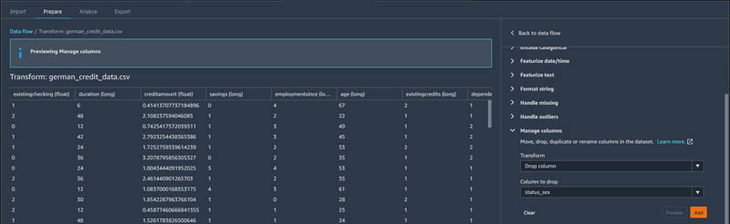
Data Wrangler contains numerous built-in data transformations so you can quickly clean, normalize, transform, and combine features. You can use these built-in data transformations without writing any code, or you can write custom transforms to make additional changes to the dataset such as encoding string categorical variables to specific numerical values.
- In the data flow view, choose the plus sign and choose Add transform.
A new view appears that shows the first few lines of the dataset, as well as a list of over 300 built-in transforms. Let’s start with modifying the status_sex column. This column contains two values: sex and marital status. We first split the string into a list of two values separated by the delimiter : .
- Choose Search and Edit.
- On the Transform menu, choose Split string by delimiter.
- For Input column, choose the
status_sex. - For Delimiter, enter
:. - For Output column, enter a name (for this post, we use
vec).
We can further flatten this column in a later step.
- Choose Preview to review the changes.
- Choose Add.

- To flatten the column
vecwe just created, we can apply a Manage vectors transformation and choose Flatten.
The outputs are two columns: sex_split_0, the Sex column, and sex_split_1, the Marital Status column.

- To easily identify the features, we can rename these two columns to
sexandmarital_statususing the Manage columns transformation by choosing Rename column.

The current credit risk classification is indicated by string values. Low risk means that the user has good credit, and high risk means that the user has bad credit. We need to encode this target or label variable as a numeric categorical variable where 0 indicates low risk and 1 indicates high risk.
- To do that, we choose Encode categorical and choose the transform Ordinal encode.
- Output this revised feature to the output column target.
The classification column now indicates 0 for low risk and 1 for high risk.

Next, let’s encode the other categorical string variables.
- Starting with
existingchecking, we can again use Ordinal encode if we consider the categories no account, none, little, and moderate to have an inherent order.

- For greater control over the encoding of ordinal variables, you can choose Custom Transform and use Python (Pandas) to create a new custom transform for the dataset.
Starting with savings, we represent the amount of money available in a savings account with the following map: {'unknown': 0 ,little': 1, 'moderate': 2, 'high': 3, 'very high': 4}.
When you create custom transforms using Python (Pandas), the DataFrame is referenced as df.
- Enter the following code into the code editor cell:
- We do the same for
employmentsince:

For more information about encoding categorical variables, see Custom Formula.
Other categorical variables that don’t have an inherent order also need to be transformed. We can use the Encode Categorical transform to one-hot encode these nominal variables. We one-hot encode housing, job, sex, and marital_status.
- Let’s start by encoding
housingby choosing One-hot encode on the Transform drop-down menu. - For Output style¸ choose Columns.

- Repeat for the remaining three nominal variables:
job,sex, andmarital_status.
After we encode all the categorical variables, we can address the numerical values. In particular, we can scale the numerical values in order to improve the performance of our future ML model.
- We do this by again choosing Add Transform and then Process numeric.
- From here you have the option of selecting between standard, robust, min-max, or max absolute scalars.

Before exporting the data, I remove the original string categorical columns that I encoded to numeric columns, so that our feature dataset contains only numbers, and therefore is machine-readable for training ML models.
- Choose Manage columns and choose the transform Drop column.
- Drop all the original categorical columns that contain string values such as
status_sex,risk, and the temporary columnvec.
As a final step, some ML libraries, such as XGBoost, expect the first column in the dataset to be the label or target variable.
- Use the Manage columns transform to move the target variable to the first column in the dataset.

We used custom and built-in transforms to create a training dataset that is ready for training an ML model. One tip for building out a data flow is to take advantage of the Previous steps tab in the right pane to walk through each step and view how the table changes after each transform. To change a step that is upstream, you have to delete all the downstream steps as well.
Further analysis and integration
In this section, we discuss opportunities for further data analysis and integration with SageMaker features.
Detect bias with Amazon SageMaker Clarify
Let’s explore Data Wrangler’s integration with other SageMaker features. In addition to the data analysis options available within Data Wrangler, you can also use Amazon SageMaker Clarify to detect potential bias during data preparation, after model training, and in your deployed model. In many use cases for detecting and analyzing bias in data and models, Clarify can be a great asset, including this credit application use case.
In this use case, we use Clarify to check for class imbalance and bias against one feature: sex. Clarify is integrated into Data Wrangler as part of the analysis capabilities, so we can easily create a bias report by adding a new analysis, choosing our target column, and selecting the column we want to analyze for bias. In this case, we use the sex column as an example, but you could continue to explore and analyze bias for other columns.

The bias report is generated by Clarify that operates within Data Wrangler. This report provides the following default metrics: class imbalance, difference in positive proportions in labels, and Jensen-Shannon Divergences. A short description provides instructions on how to read each metric. In our example, the report indicates that the data may be imbalanced. We should consider using sampling methods to correct this imbalance in our training data. For more information about Clarify capabilities and how to create a Clarify processing job using the SageMaker Python SDK, see New – Amazon SageMaker Clarify Detects Bias and Increases the Transparency of Machine Learning Models.
Support rapid model prototyping with Data Wrangler Quick Model visualization
Let’s now use Data Wrangler’s Quick Model analysis, which allows you to quickly evaluate your data and produce importance scores for each potential feature that you may consider including in an ML model, now that your data preparation data flow is complete. The Quick Model analysis gives you a feature importance score for each variable in the data, indicating how useful a feature is at predicting the target label.
This Quick Model also provides an overall model score. For a classification problem, such as our use case of predicting high or low credit risk, the Quick Model also provides an F1 score. This gives an indication of potential model fit using the data as you’ve prepared it in your complete data flow. For regression problems, the model provides a mean squared error (MSE) score. In the following screenshot, we can see which features contribute most to the predicted outcome: existing checking, credit amount, duration of loan, and age. We can use this information to inform our model development approach or make additional adjustments to our data flow, such as dropping additional columns with low feature importance.

Use Data Wrangler data flows in ML deployments
After you complete your data transformation steps and analysis, you can conveniently export your data preparation workflow flow. When you export your data flow, you have the option of exporting to the following:
- A notebook running the data flow as a Data Wrangler job – Exporting as a Data Wrangler job and running the resulting notebook takes the data processing steps defined in your .flow file and generates a SageMaker processing job to run these steps on your entire source dataset, providing a way to save processed data as a CSV or Parquet file to Amazon S3.
- A notebook running the data flow as an Amazon SageMaker Pipelines workflow – With Amazon SageMaker Pipelines, you can create end-to-end workflows that manage and deploy SageMaker jobs responsible for data preparation, model training, and model deployment. By exporting your Data Wrangler flow to Pipelines, a Jupyter notebook is created that, when run, defines a data transformation pipeline following the data processing steps defined in your .flow file.
- Python code replicating the steps in the Data Wrangler data flow – Exporting as a Python file enables you to manually integrate the data processing steps defined in your flow into any data processing workflow.
- A notebook pushing your processed features to Feature Store – When you export to Feature Store and run the resulting notebook, your data can be processed as a SageMaker processing job, and then ingested into an online and offline feature store.

Conclusion
In this post, we explored the German credit risk dataset to understand the transformation steps needed to prepare the data for ML modeling so financial institutions can approve loans more easily. We then created ordinal and one-hot encoded features from the categorical variables, and finally scaled our numerical features—all using Data Wrangler. We now have a complete data transformation data flow that has transformed our raw dataset into a set of features ready for training an ML model to predict credit risk among credit applicants.
The options to export our Data Wrangler data flow allow us to use the transformation pipeline as a Data Wrangler processing job, create a feature store to better store and track features to be used in future modeling, or save the transformation steps as part of a complete SageMaker pipeline in your ML workflow. Data Wrangler makes it easy to work interactively on data preparation steps before transforming them into code that can be used immediately for ML model experimentation and into production.
To learn more about Amazon SageMaker Data Wrangler, visit the webpage. Give Data Wrangler a try, and let us know what you think in the comments!
About the Author
Courtney McKay is a Senior Principal with Slalom Consulting. She is passionate about helping customers drive measurable ROI with AI/ML tools and technologies. In her free time, she enjoys camping, hiking and gardening.