Streamline modeling with Amazon SageMaker Studio and the Amazon Experiments SDK

The modeling phase is a highly iterative process in machine learning (ML) projects, where data scientists experiment with various data preprocessing and feature engineering strategies, intertwined with different model architectures, which are then trained with disparate sets of hyperparameter values. This highly iterative process with many moving parts can, over time, manifest into a tremendous headache in terms of keeping track of the design decisions applied in each iteration and how the training and evaluation metrics of each iteration compare to the previous versions of the model.

While your head may be spinning by now, fear not! Amazon SageMaker has a solution!

This post walks you through an end-to-end example of using Amazon SageMaker Studio and the Amazon SageMaker Experiments SDK to organize, track, visualize, and compare our iterative experimentation with a Keras model. Although this use case is specific to Keras framework, you can extend the same approach to other deep learning frameworks and ML algorithms.

Amazon SageMaker is a fully managed service, created with the goal of democratizing ML by empowering developers and data scientists to quickly and cost-effectively build, train, deploy, and monitor ML models.

What Is Amazon SageMaker Experiments?

Amazon SageMaker Experiments is a capability of Amazon SageMaker that lets you effortlessly organize, track, compare, and evaluate your ML experiments. Before we dive into the hands-on exercise, let’s first take a step back and review the building blocks of an experiment and their referential relationships. The following diagram illustrates these building blocks.

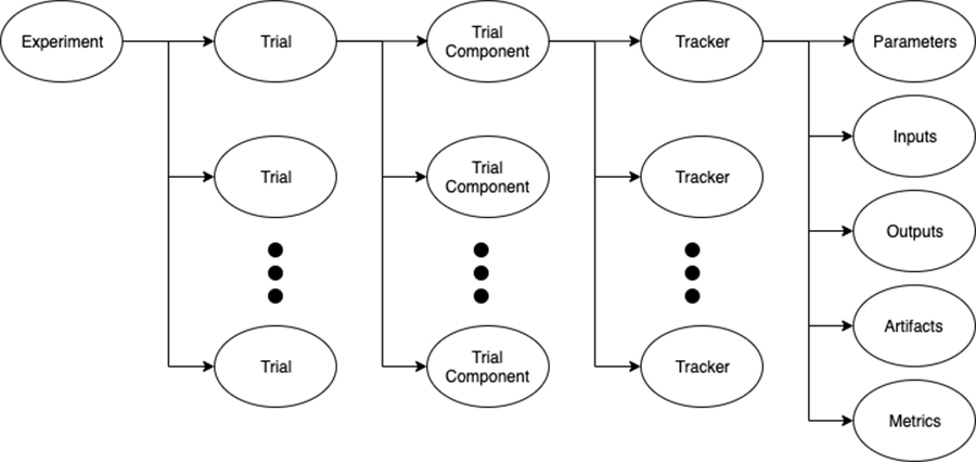
Figure 1. The building blocks of Amazon SageMaker Experiments

Amazon SageMaker Experiments is composed of the following components:

• Experiment – An ML problem that we want to solve. Each experiment consists of a collection of trials.
• Trial – An iteration of a data science workflow related to an experiment. Each trial consists of several trial components.
• Trial component – A stage in a given trial. For instance, as we see in our example, we create one trial component for the data preprocessing stage and one trial component for model training. In a similar fashion, we can also add a trial component for any data postprocessing.
• Tracker – A mechanism that records various metadata about a particular trial component, including any parameters, inputs, outputs, artifacts, and metrics. A tracker can be linked to a particular training component to assign the collected metadata to it.

Now that we’ve set a rock-solid foundation on the key building blocks of the Amazon SageMaker Experiments SDK, let’s dive into the fun hands-on component.

Prerequisites

You should have an AWS account and a sufficient level of access to create resources in the following AWS services:

• Amazon SageMaker
• Amazon Simple Storage Service (Amazon S3)
• Amazon CloudWatch

Solution overview

As part of this post, we walk through the following high-level steps:

1. Environment setup
2. Data preprocessing and feature engineering
3. Modeling with Amazon SageMaker Experiments
4. Training and evaluation metric exploration
5. Environment cleanup

Setting up the environment

We can set up our environment in a few simple steps:

1. Clone the source code from the GitHub repo, which contains the complete demo, into your Amazon SageMaker Studio environment.
2. Open the included Jupyter notebook and choose the Python 3 (TensorFlow 2 CPU Optimized)
3. When the kernel is ready, install sagemaker-experiments package, which enables us to work with the Amazon SageMaker Experiments SDK, and s3fs package, to enable our pandas dataframes to easily integrate with objects in Amazon S3.
4. Import all required packages and initialize the variables.

The following screenshot shows the environment setup.

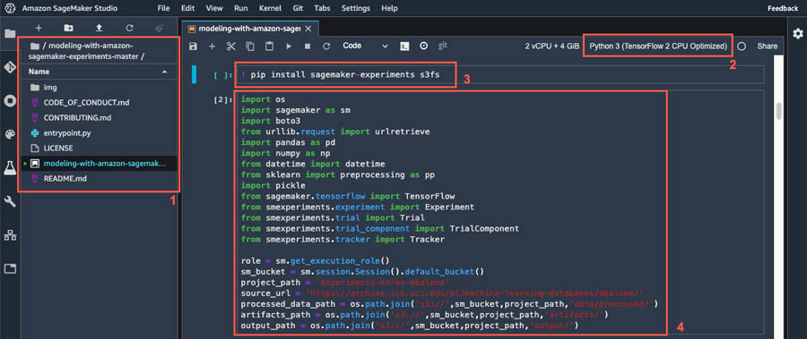
Figure 2. Environment Setup

Data preprocessing and feature engineering

Excellent! Now, let’s dive into data preprocessing and feature engineering. In our use case, we use the abalone dataset from the UCI Machine Learning Repository.

Run the steps in the provided Jupyter notebook to complete all data preprocessing and feature engineering. After your data is preprocessed, it’s time for us to seamlessly capture our preprocessing strategy! Let’s create an experiment with the following code:

sm = boto3.client('sagemaker') 
ts = datetime.now().strftime('%Y-%m-%d-%H-%M-%S-%f')

abalone_experiment = Experiment.create(
    experiment_name = 'predict-abalone-age-' + ts,
    description = 'Predicting the age of an abalone based on a set of features describing it',
    sagemaker_boto_client=sm)

Now, we can create a Tracker to describe the Pre-processing Trial Component, including the location of the artifacts:

with Tracker.create(display_name='Pre-processing', sagemaker_boto_client=sm, artifact_bucket=sm_bucket, artifact_prefix=artifacts_path) as tracker:
    tracker.log_parameters({
        'train_test_split': 0.8
    })
    tracker.log_input(name='raw data', media_type='s3/uri', value=source_url)
    tracker.log_output(name='preprocessed data', media_type='s3/uri', value=processed_data_path)
    tracker.log_artifact(name='preprocessors', media_type='s3/uri', file_path='preprocessors.pickle')
    
processing_component = tracker.trial_component

Fantastic! We now have our experiment ready and we’ve already done our due diligence to capture our data preprocessing strategy. Next, let’s dive into the modeling phase.

Modeling with Amazon SageMaker Experiments

Our Keras model has two fully connected hidden layers with a variable number of neurons and variable activation functions. This flexibility enables us to pass these values as arguments to a training job and quickly parallelize our experimentation with several model architectures.

We have mean squared logarithmic error defined as the loss function, and the model is using the Adam optimization algorithm. Finally, the model tracks mean squared logarithmic error as our metric, which automatically propagates into our training trial component in our experiment, as we see shortly:

def model(x_train, y_train, x_test, y_test, args):
    """Generate a simple model"""
    model = Sequential([
                Dense(args.l1_size, activation=args.l1_activation, kernel_initializer='normal'),
                Dense(args.l2_size, activation=args.l2_activation, kernel_initializer='normal'),
                Dense(1, activation='linear')
    ])

    model.compile(optimizer=Adam(learning_rate=args.learning_rate),
                  loss='mean_squared_logarithmic_error',
                  metrics=['mean_squared_logarithmic_error'])
    model.fit(x_train, y_train, batch_size=args.batch_size, epochs=args.epochs, verbose=1)
    model.evaluate(x_test,y_test,verbose=1)

    return model

Fantastic! Follow the steps in the provided notebook to define the hyperparameters for experimentation and instantiate the TensorFlow estimator. Finally, let’s start our training jobs and supply the names of our experiment and trial via the experiment_config dictionary:

abalone_estimator.fit(processed_data_path,
                        job_name=job_name,
                        wait=False,
                        experiment_config={
                                        'ExperimentName': abalone_experiment.experiment_name,
                                        'TrialName': abalone_trial.trial_name,
                                        'TrialComponentDisplayName': 'Training',
                                        })

Exploring the training and evaluation metrics

Upon completion of the training jobs, we can quickly visualize how different variations of the model compare in terms of the metrics collected during model training. For instance, let’s see how the loss has been decreasing by epoch for each variation of the model and observe the model architecture that is most effective in decreasing the loss:

1. Choose the Amazon SageMaker Experiments List icon on the left sidebar.
2. Choose your experiment to open it and press Shift to select all four trials.
3. Choose any of the highlighted trials (right-click) and choose Open in trial component list.
4. Press Shift to select the four trial components representing the training jobs and choose Add chart.
5. Choose New chart and customize it to plot the collected metrics that you want to analyze. For our use case, choose the following:
   1. For Data type¸ choose Time series.
   2. For Chart type¸ choose Line.
   3. For X-axis dimension, choose epoch.
   4. For Y-axis, choose loss_TRAIN_last.

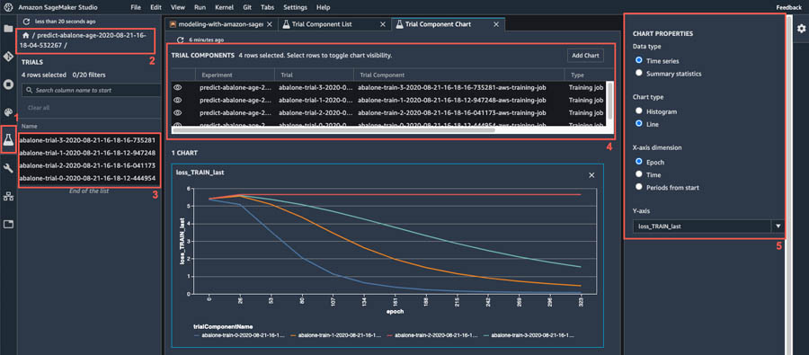
Figure 3. Generating plots based on the collected model training metrics

Wow! How quick and effortless was that?! I encourage you to further explore plotting various other metrics on your own. For instance, you can choose the Summary data type to generate a scatter plot and explore if there is a relationship between the size of the first hidden layer in your neural network and the mean squared logarithmic error. See the following screenshot.

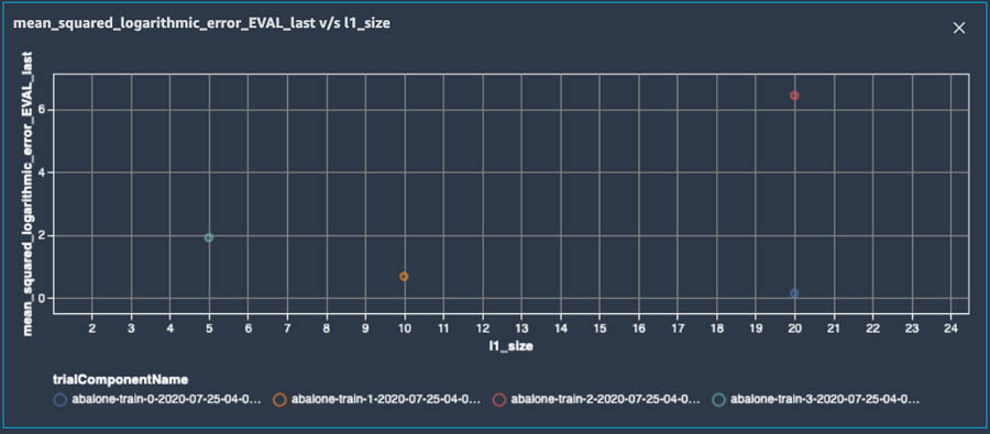
Figure 4. Plot of the relationship between the size of the first hidden layer in the neural network and Mean-Squared Logarithmic Error during model evaluation

Next, let’s choose our best-performing trial (abalone-trial-0). As expected, we see two trial components. One represents our data Pre-processing, and the other reflects our model Training. When we open the Training trial component, we see that it contains all the hyperparameters, input data location, Amazon S3 location of this particular version of the model, and more.

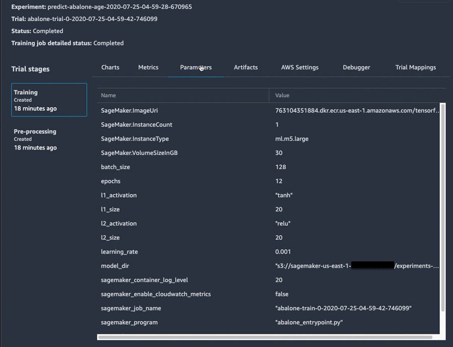
Figure 5. Metadata about model training, automatically collected by Amazon SageMaker Experiments

Similarly, when we open the Pre-processing component, we see that it captures where the source data came from, where the processed data was stored in Amazon S3, and where we can easily find our trained encoder and scalers, which we’ve packaged into the preprocessors.pickle artifact.

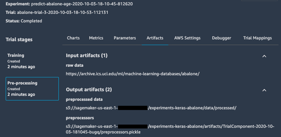
Figure 6. Metadata about data pre-processing and feature engineering, automatically collected by Amazon SageMaker Experiments

Cleaning up

What a fun exploration this has been! Let’s now clean up after ourselves by running the cleanup function provided at the end of the notebook to hierarchically delete all elements of the experiment that we created in this post:

abalone_experiment.delete_all('--force')

Conclusion

You have now learned to seamlessly track the design decisions that you made during data preprocessing and model training, as well as rapidly compare and analyze the performance of various iterations of your model by using the tracked metrics of the trials in your experiment.

I hope that you enjoyed diving into the intricacies of the Amazon SageMaker Experiments SDK and exploring how Amazon SageMaker Studio smoothly integrates with it, enabling you to lose yourself in experimentation with your ML model without losing track of the hard work you’ve done! I highly encourage you to leverage the Amazon SageMaker Experiments Python SDK in your next ML engagement and I invite you to consider contributing to the further evolution of this open-sourced project.

About the Author

Ivan Kopas is a Machine Learning Engineer for AWS Professional Services, based out of the United States. Ivan is passionate about working closely with AWS customers from a variety of industries and helping them leverage AWS services to spearhead their toughest AI/ML challenges. In his spare time, he enjoys spending time with his family, working out, hanging out with friends and diving deep into the fascinating realms of economics, psychology and philosophy.