AWS Physical AI Blog
Build L1–4 Industrial Digital Twins with OpenUSD and SDMA on AWS
Introduction
Digital twins shift manufacturing teams from reactive maintenance to predictive operations. A production-grade twin goes beyond static 3D. It ingests live data, predicts failures, and self-corrects as equipment ages. In this post, you’ll learn how to architect a multi-level digital twin on AWS using Universal Scene Description (OpenUSD) for scene composition and Spatial Data Management on AWS (SDMA) for single source of truth for spatial assets. The approach is open-standard, incrementally deployable, and runs on managed services. Each level delivers standalone value and adds capability without modifying the level below. This guide implements the full L1–L4 pattern with Amazon Simple Storage Service (Amazon S3) as the scene store so you can deploy every level end to end, and it points out exactly where SDMA slots in as the production upgrade path for governed, versioned asset management.
Digital twin maturity levels
AWS describes a four-level digital twin maturity framework based on the Digital Twin Consortium’s capability scale. Each level builds on the previous, so you invest incrementally.
- Level 1: Descriptive: Represents the physical system through engineering designs, CAD/BIM models, 3D visualizations, and as-built documentation. What does the system look like?
- Level 2: Informative: Connects the digital model to live data from IoT sensors, SCADA (Supervisory Control and Data Acquisition) systems, or historian databases. What is happening right now?
- Level 3: Predictive: Adds physics-based simulations or machine learning models to forecast future behavior. What will happen next?
- Level 4: Living: Continuously updates model parameters using real-world operational data to self-calibrate. How should the system adapt?
Each level depends on the one below it. You need L1 geometry before L2 can bind data, and reliable L2 data before L3 predictions are meaningful.
Why OpenUSD for industrial digital twins?
OpenUSD, developed by Pixar and governed by the Alliance for OpenUSD (AOUSD), is the standard framework for composing complex 3D scenes. OpenUSD unifies CAD data, simulation assets, and IoT telemetry into a single physically accurate representation, eliminating format silos between engineering and operations teams. Its layer-based architecture lets teams own and update independent scene layers without coordination overhead, while IoT data and simulation results overlay on base geometry non-destructively (remove the overlay and the scene reverts to its original state). Attributes support time-sampled values, so predictions and historical state store as playable timelines within the scene. Variant sets allow multiple named states, such as per-batch calibration parameters, to coexist in one file with full version history. Together, these capabilities make OpenUSD a foundation for physically accurate simulation, AI model training, and autonomous industrial operations.
Introducing Spatial Data Management on AWS (SDMA)
SDMA manages large-scale spatial assets (point clouds, 3D models, geospatial imagery) in a secure, centralized cloud environment. It provides versioning, metadata enrichment, and governance across the entire lifecycle of physical assets.
It consists of three layers:
- Client layer: A Spatial Data Portal (web and desktop applications), REST APIs through Amazon API Gateway, Python CLI tools, and direct Amazon S3 access for large file uploads and downloads.
- Control and data plane: Amazon API Gateway and AWS Lambda for business logic, Amazon S3 with content-addressable storage for spatial assets, Amazon DynamoDB for metadata, and Amazon OpenSearch Serverless for full-text search.
- Integration layer: Amazon EventBridge, Amazon Simple Queue Service (Amazon SQS), and pre-built connectors for external systems including digital twin platforms, GIS tools, and CAD applications. Custom transformation connectors use AWS Deadline Cloud for compute-intensive processing such as format conversion, 3D rendering, and metadata extraction.
- OpenUSD and SDMA are complementary. OpenUSD is the composable scene description. SDMA is the governed data fabric that stores, versions, and serves those assets across their lifecycle. The following diagram shows how OpenUSD, SDMA, and AWS services combine across the four maturity levels:
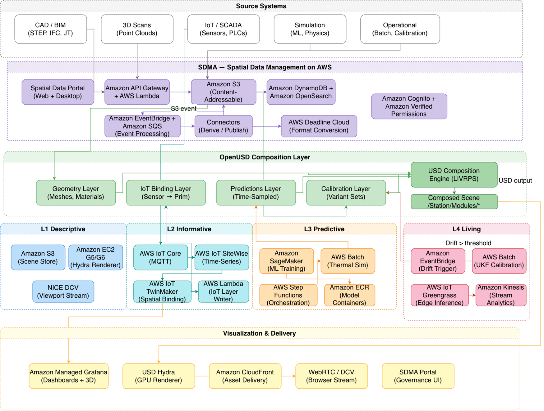
Figure 1: OpenUSD and SDMA reference architecture for L1–L4 digital twins on AWS
AWS IoT TwinMaker (shown under L2 in the diagram) is a strong fit for L1–L2 operational dashboards that bind live telemetry to a scene. This architecture goes further: it uses OpenUSD for non-destructive scene composition, adds physics-based L3 forecasting on AWS Batch, and closes an autonomous L4 recalibration loop. You can use AWS IoT TwinMaker for the dashboard layer and this pattern for the predictive and living layers.
Solution overview: an EV battery assembly station twin
This walkthrough applies the architecture to an EV battery assembly station. The station assembles individual cell modules into packs. It includes fixture trays, torque tools, alignment jigs, cooling manifolds, and sensors measuring voltage, temperature, torque, and pressure. Multiple sensor types exercise L2. Measurable thermal degradation drives L3 predictions. Batch-to-batch chemistry variation triggers L4 recalibration.
Solution Architecture:
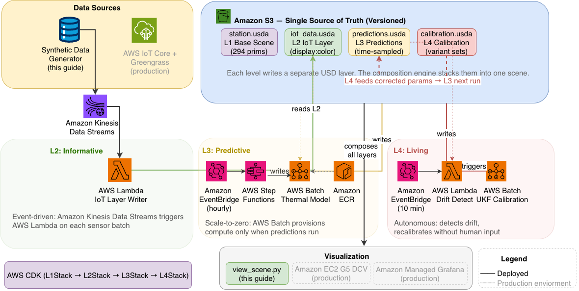
Figure 2: EV Battery Assembly Station: Digital Twin Architecture (L1–L4)
The implementation uses Amazon S3 for versioned scene storage, Amazon Kinesis Data Streams for real-time sensor ingestion, AWS Lambda for event-to-USD transformation, AWS Batch with Amazon Elastic Container Registry (Amazon ECR) for containerized simulation (scales to zero between runs), and AWS Step Functions with Amazon EventBridge for orchestration and drift-triggered recalibration. All infrastructure is defined in AWS Cloud Development Kit (AWS CDK) for repeatable deployment.
This guide uses Amazon S3 for scene storage and a synthetic data generator for sensor input. In production, substitute SDMA for governed asset lifecycle management and AWS IoT Core or AWS IoT SiteWise for real sensor feeds. For GPU-rendered streaming viewports, add Amazon Elastic Compute Cloud (Amazon EC2) G5 instances with NICE DCV.
| Component | This guide | In production |
|---|---|---|
| Scene / asset store | Amazon S3 (versioned bucket) | SDMA (governed, versioned assets) |
| Sensor input | Synthetic data generator | AWS IoT Core / AWS IoT SiteWise |
| Scene viewer | Local USD viewer | Amazon EC2 G5 + NICE DCV streaming |
| Prediction compute | AWS Batch (c6i.large) | AWS Batch / your simulation engine |
| Orchestration | AWS Step Functions + Amazon EventBridge | AWS Step Functions + Amazon EventBridge |
Table 1: Components used in this guide and their production equivalents
Using SDMA in production
To deploy SDMA and use it as the governed asset store for this architecture, see the Spatial Data Management on AWS deployment guide. Once deployed, substitute the Amazon S3 bucket references in this guide with SDMA’s asset API. SDMA adds: content-addressable versioning (every scene change tracked with full rollback), metadata enrichment and full-text search across spatial assets, role-based access control with audit trails, and event-driven connectors that trigger downstream pipelines (like L3 predictions) when assets change. The companion branch of this repository includes a complete SDMA integration that replaces the Amazon S3-only flow shown here.
Prerequisites:
The complete source code is available at: https://github.com/aws-samples/sample-physical-ai-spatial-intelligence
Prerequisites: AWS account, Python 3.12+, Node.js 22+, Docker, and AWS CLI configured with appropriate permissions.
git clone git@github.com:aws-samples/sample-physical-ai-spatial-intelligence.gitcd ev-battery-digital-twinpython3 -m venv .venv && source .venv/bin/activateexport CDK_DEFAULT_ACCOUNT=$(aws sts get-caller-identity --query Account --output text --region us-east-1)bash setup.shexport CDK_DEFAULT_REGION=us-east-1; cd infrastructure; cdk bootstrap; cd ..
The setup script checks prerequisites, installs Python and CDK dependencies, and verifies OpenUSD imports. From git clone to all four levels operational takes roughly 30 minutes, most of it unattended CDK deployment and first-run AWS Batch provisioning.
Level 1 – Descriptive twin: establishing the digital foundation
The L1 twin creates a comprehensive digital description of your physical assets. This is where OpenUSD and SDMA form the foundational data layer.
In production, you ingest CAD files (STEP, IFC, Revit), BIM models, and point cloud scans into SDMA, whose content-addressable storage provides version control and data integrity. SDMA’s transformation connectors convert proprietary formats into OpenUSD. For this guide, you generate the scene programmatically to demonstrate the same composition principles.
Step 1: Compose the USD scene
python scene/compose_station.py
This generates station.usda: a USD scene graph with 294 prims organized into structure, modules, robotics, tooling, electrical, cooling, operator controls, safety, and factory floor.
Each sensor-equipped prim stores an asset_id in its customData block. This is the binding contract between geometry and live data. Subsequent levels use these bindings to attach sensor readings, predictions, and calibration parameters to the correct 3D component.
Verify the bindings exist:
grep "asset_id" station.usda | head -3
You should see asset_id = “cell_module_01” through cell_module_12 confirming each module is tagged for L2 data binding.
Step 2: View the scene
python view_scene.py station.usda
An interactive viewport opens. Components render with factory-standard colors: orange for the robot arm, blue for cell modules, copper for busbars, yellow for safety markings. Rotate with left-click drag, zoom with scroll, pan with middle-click.
Step 3: Deploy and upload scene to Amazon S3
cd infrastructurecdk deploy L1Stack --require-approval never
export SCENE_BUCKET=$(aws cloudformation describe-stacks \--stack-name L1Stack \--query "Stacks[0].Outputs[?OutputKey=='SceneBucketName'].OutputValue" \--output text)
L1Stack deploys a versioned Amazon S3 bucket. Every scene change is tracked with full rollback capability.
cd ..aws s3 cp station.usda s3://$SCENE_BUCKET/station.usda
The scene is now the single source of truth in the cloud. All subsequent levels write layers that reference prims defined here.
Note: In production, you can add a GPU-rendered streaming viewport (Amazon EC2 G5 with NICE DCV) so operators view the scene from a browser without local software. This is not required for this guide.
Level 2 – Informative twin: connecting to real-time data
L2 connects live sensor data to the scene. When a sensor record lands in the Amazon Kinesis Data Streams, AWS Lambda triggers, classifies the reading, and writes a USD override layer to Amazon S3 that changes module colors without modifying the base geometry. An operator sees which modules are nominal (green), warning (yellow), or fault (red).
The data flow: sensor readings arrive in an Amazon Kinesis Data Stream as JSON records. AWS Lambda triggers on each batch, classifies each module against thresholds (voltage < 3.4V = warning, temperature > 42°C = fault), and writes a USD override layer to Amazon S3. The override uses USD’s over statement to set a display:color attribute on each module prim. The base station.usda is never touched. Removing the IoT layer and the scene reverts to L1.
over "Station" {over "Modules" {over "Module_03" {float3 display:color = (0.9, 0.7, 0.1)double iot:temperature = 38.5string iot:status = "warning"}}}
The pipeline from Amazon Kinesis onward is production-ready. In production, you replace the synthetic generator with AWS IoT Core routing real sensor data to the same Amazon Kinesis stream. The AWS Lambda, the override layer format, and the Amazon S3 output remain unchanged.
Step 1: Deploy streaming infrastructure
cd infrastructurecdk deploy L2Stack --require-approval never
Verify the stream is active:
aws kinesis describe-stream-summary --stream-name ev-battery-sensors \--query "StreamDescriptionSummary.{Status:StreamStatus,Shards:OpenShardCount}" \--output table
L2Stack creates an Amazon Kinesis Data Stream, an AWS Lambda function that transforms sensor records into a USD override layer, and the event source mapping between them.
Step 2: Start the data generator
Terminal 1 (leave running):
python data_generator/generate_sensor_data.py \--kinesis --stream-name $STREAM_NAME --interval 5
Readings publish every 5 seconds for 12 modules. Each record carries module_id, voltage, temperature, torque, pressure, and a status classification (nominal, warning, or fault).
Step 3: Verify the USD layer update
Terminal 2 (wait 30 seconds after generator starts):
# Check AWS Lambda logsaws logs tail $LAMBDA_LOG --since 2m --region $AWS_DEFAULT_REGION
# Verify layer exists in Amazon S3export SCENE_BUCKET=$(aws cloudformation describe-stacks \--stack-name L1Stack \--query "Stacks[0].Outputs[?OutputKey=='SceneBucketName'].OutputValue" \--output text --region $AWS_DEFAULT_REGION)echo "SCENE_BUCKET: $SCENE_BUCKET"aws s3 ls s3://$SCENE_BUCKET/layers/ --region $AWS_DEFAULT_REGION
# Download and viewaws s3 cp s3://$SCENE_BUCKET/layers/iot_data.usda ./layers/iot_data.usda --region $AWS_DEFAULT_REGIONpython view_scene.py twin_l2.usda
Modules display green (nominal), yellow (warning), or red (fault) based on sensor thresholds. The base station.usda is never modified. The IoT layer stacks on top non-destructively.
Level 3 – Predictive twin: modeling future behavior
L3 reads the current sensor state from L2 and predicts thermal resistance growth per module into the future. The twin shows which modules will cross the failure threshold and when, enabling maintenance decisions before failures occur.
The data flows directly from L2 to L3. The AWS Lambda in L2 writes current temperatures to layers/iot_data.usda in Amazon S3. The prediction model reads that same file, applies a thermal degradation equation to each module’s current temperature and cycle count, and writes the result to layers/predictions.usda as time-sampled attributes. Each hour is a frame. Colors shift green to yellow to red as predicted resistance approaches the failure threshold. If a module runs hotter today, tomorrow’s prediction reflects that automatically.
The predictions layer stores each module’s forecast as USD time samples, one frame per hour:
over "Station" {over "Modules" {over "Module_12" {double prediction:thermal_resistance.timeSamples = {0: 0.016884,24: 0.020074,48: 0.023844,72: 0.028037,}custom double prediction:hours_to_threshold = 55}}}
The thermal model in this guide uses a physics-based equation. The same AWS Batch infrastructure runs any model you provide like scikit-learn, COMSOL, or a custom FEA solver. You just have to swap the container.
R_thermal(t) = R_0 * (1 + alpha * cycles * exp(beta * (T - T_ref)))
where R_0 is the baseline resistance, cycles is the elapsed duty cycles, T is the operating temperature, and T_ref is the reference temperature. alpha is the per-cycle degradation rate and beta is the sensitivity of resistance growth to temperature. L4 calibrates alpha and beta from observed data.
Step 1: Download sensor state and run prediction locally
# Download latest sensor state from L2aws s3 cp s3://$SCENE_BUCKET/layers/iot_data.usda ./layers/iot_data.usda --region $AWS_DEFAULT_REGION
# Run prediction (reads L2 sensor state as input)python thermal_model/thermal_simulation.py
# Write predictions to USD time samplespython thermal_model/write_predictions_usd.py
# View predicted state at different hourspython view_scene.py twin_l3.usda --timecode 0
View the scene at different timecodes to see the prediction timeline: at timecode 0 all modules are green (below threshold), at timecode 10 modules 10–12 turn orange (approaching threshold), and at timecode 18 most modules are red (threshold crossed). Replace the timecode value in the command above to scrub through the 72-hour forecast.
Step 2: Deploy L3 infrastructure
cd infrastructurecdk deploy L3Stack --require-approval nevercd ..
export STATE_MACHINE_ARN=$(aws cloudformation describe-stacks \--stack-name L3Stack \--query "Stacks[0].Outputs[?OutputKey=='StateMachineArn'].OutputValue" \--output text --region $AWS_DEFAULT_REGION)
L3Stack deploys an AWS Batch compute environment (c6i.large, scales to zero between runs), an AWS Step Functions state machine, an Amazon ECR container image, and an Amazon EventBridge rule that triggers predictions hourly. Between runs, compute costs are near zero.
Step 3: Trigger and verify prediction on AWS
Trigger the prediction:
aws stepfunctions start-execution \--state-machine-arn $STATE_MACHINE_ARN \--name "prediction-$(date +%s)" \--region $AWS_DEFAULT_REGION
The Step Functions state machine submits a Batch job. Batch provisions a c6i.large instance, pulls the container from Amazon ECR, and runs the prediction model. The container downloads the latest L2 sensor state from Amazon S3, runs the thermal model, writes predictions.usda back to Amazon S3, and terminates. First run takes 3-5 minutes (instance provisioning). Subsequent runs complete in under 2 minutes.
Verify execution completed:
aws stepfunctions list-executions \--state-machine-arn $STATE_MACHINE_ARN \--max-results 1 \--query "executions[0].{Name:name,Status:status}" \--output table --region $AWS_DEFAULT_REGIONExpected: Status = SUCCEEDED
Verify predictions written to Amazon S3:
aws s3api head-object --bucket $SCENE_BUCKET --key layers/predictions.usda \--query "{LastModified:LastModified,Size:ContentLength}" \--output table --region $AWS_DEFAULT_REGIONExpected: LastModified within the last few minutes, Size ~118KB.
Download and view:
aws s3 cp s3://$SCENE_BUCKET/layers/predictions.usda ./layers/predictions.usda --region $AWS_DEFAULT_REGIONpython view_scene.py twin_l3.usda --timecode 10
The viewer shows modules 10-12 in orange and modules 1-5 in green. The model produced identical results running locally and on Batch because the same container image and the same L2 sensor data in Amazon S3 were used in both cases. Amazon EventBridge triggers this every hour automatically.
Level 4 – Living twin: self-calibrating and autonomous
L4 closes the feedback loop. It reads what L2 observed and what L3 predicted. When the error between them exceeds a threshold, it recalibrates the model parameters automatically.
This makes the twin self-correcting. When a new cell chemistry batch arrives or equipment ages, the twin detects drift and adapts. Predictions stay accurate across the life of the asset without manual retuning.
Under the hood, calibration uses an Unscented Kalman Filter (UKF). The UKF treats the thermal model’s parameters (alpha, beta, and T_factor) as hidden state and estimates them from the gap between L2 observed temperatures and L3 predictions. A UKF is used rather than a linear Kalman filter because thermal degradation is nonlinear: it propagates a set of sigma points through the model to capture that nonlinearity without hand-derived Jacobians. Physically, alpha is the per-cycle degradation rate and beta is how strongly resistance growth responds to temperature, so recovering them re-tunes both how fast and how heat-sensitively a given battery batch ages.
Step 1: Verify calibration locally
The calibration reads from both L2 and L3:
# Ensure L2 and L3 outputs exist locally (from previous steps)# layers/iot_data.usda → L2 actual temperatures# predictions.json → L3 predicted resistance
# Run calibrationPYTHONPATH=. python calibration/ukf_calibration.py
Output:
Mean drift: 0.003180 K/W (threshold: 0.003000 K/W)⚠️ Drift exceeds threshold. Recalibration triggered.
Calibration result:Error before: 0.004454 (Supplier A)Error after: 0.002580 (Supplier B)alpha: 0.0002 → 0.000454
The UKF detected that Supplier B cells degrade faster than the model expected (alpha nearly doubled). After calibration, prediction error drops. The next L3 run using these parameters will produce more accurate forecasts.
Store the calibration as a USD variant:
PYTHONPATH=. python calibration/write_variant_usd.py
Output:
Calibration variant added: supplier_B_week_3 (layers/calibration.usda, alpha=0.000454, beta=1.2963)
Each calibration creates a named variant in layers/calibration.usda. Engineers switch between variants to compare how the model behaves with different parameter sets across supplier batches.
Each variant captures a full parameter set as a named USD variant selection:
over "Station" {over "ThermalModel" (variants = { string calibration_state = "supplier_B_week_3" }prepend variantSets = "calibration_state") {variantSet "calibration_state" = {"supplier_B_week_3" {custom double calibration:alpha = 0.000390custom double calibration:beta = 1.286custom double calibration:T_factor = 0.025919}}}}
Step 2: Deploy L4 infrastructure
cd infrastructurecdk deploy L4Stack --require-approval nevercd ..
L4Stack deploys:
- A drift detector AWS Lambda (triggered every 10 minutes by Amazon EventBridge)
- A UKF calibration Batch job definition
- AWS Identity and Access Management (IAM) roles granting access to read L2/L3 data and write calibration results in Amazon S3
The drift detector reads layers/iot_data.usda and predictions.json from Amazon S3 every 10 minutes. If prediction error exceeds 0.003 K/W, it submits a calibration Batch job.
Step 3: Verify the autonomous loop
Simulate drift by writing an error metric to Amazon S3:
echo '{"mean_error": 0.005}' > /tmp/prediction_error.jsonaws s3 cp /tmp/prediction_error.json s3://$SCENE_BUCKET/metrics/prediction_error.json --region $AWS_DEFAULT_REGION
Invoke the drift detector:
DRIFT_LAMBDA=$(aws lambda list-functions --region $AWS_DEFAULT_REGION \--query "Functions[?contains(FunctionName,'Drift')].FunctionName" --output text)aws lambda invoke --function-name $DRIFT_LAMBDA /tmp/response.json --region $AWS_DEFAULT_REGIONcat /tmp/response.json
Expected:
{"drift_detected": true, "error": 0.005, "action": "calibration_triggered"}
Wait 3-5 minutes for AWS Batch to provision and run, then verify:
# Check calibration file written to Amazon S3aws s3api head-object --bucket $SCENE_BUCKET --key layers/calibration.usda \--query "{LastModified:LastModified,Size:ContentLength}" \--output table --region $AWS_DEFAULT_REGION
Expected: LastModified within the last few minutes.
Download and view the full twin (all 4 layers composed):
aws s3 cp s3://$SCENE_BUCKET/layers/calibration.usda ./layers/calibration.usda --region $AWS_DEFAULT_REGIONpython view_scene.py twin.usda --timecode 10
The full composite scene (twin.usda) now includes all four layers: base geometry (L1), live sensor state (L2), predictions (L3), and calibration parameters (L4). The feedback loop is closed. Amazon EventBridge fires the drift detector every 10 minutes. When conditions change, the twin self-corrects.
Cleanup
cd infrastructurecdk destroy --all --force
This removes all AWS CloudFormation stacks including Amazon S3 bucket, Amazon Kinesis stream, AWS Lambda functions, AWS Batch compute environments, AWS Step Functions state machine, Amazon EventBridge rules, Amazon ECR images, and AWS IAM roles. If you deployed SDMA separately, follow the SDMA cleanup instructions in the Spatial Data Management on AWS documentation to remove those resources.
How the levels connect
The twin is not four independent layers. It is a feedback system. L2 feeds L3. L3 and L2 together feed L4. L4 improves L3. The cycle repeats every hour.
| Level | Purpose | Key services | Data freshness |
|---|---|---|---|
| L1 Descriptive | Geometry + metadata bindings | Amazon S3, OpenUSD | Static (versioned) |
| L2 Informative | Live sensor state overlay | Amazon Kinesis, AWS Lambda, Amazon S3 | Seconds (streaming) |
| L3 Predictive | Thermal forecast | AWS Batch, AWS Step Functions, Amazon EventBridge | Hourly |
| L4 Living | Autonomous recalibration | AWS Batch, AWS Lambda, Amazon EventBridge | Event-driven (on drift) |
Table 2: Digital twin levels, their purpose, and operational cadence
Production considerations: monitoring and error handling
This guide walks the happy path, but a production deployment needs failure handling at every level. Add Amazon CloudWatch alarms on the L3 and L4 Batch job failure metrics and on AWS Lambda error and throttle metrics so operators are paged when a prediction or calibration run fails. Attach a dead-letter queue (DLQ) to the Amazon Kinesis event source mapping so sensor records that repeatedly fail transformation are captured rather than dropped. Use the AWS Step Functions state machine’s built-in Catch and Retry to absorb transient Batch failures and route unrecoverable errors to an alerting path. For L4 specifically, bound the calibrated parameters and alarm on a non-converged UKF run so a diverging fit never silently feeds back into L3.
Conclusion
You deployed a self-correcting digital twin using four composable USD layers in Amazon S3. The system ingests live data, predicts failures, recalibrates when conditions drift, and stays accurate as the physical asset ages, all on managed AWS services that scale to zero between runs. Because every layer is standard OpenUSD, the twin opens in Omniverse, Reality Composer, and other OpenUSD-compatible viewers without modification. To move to production, swap the synthetic generator for AWS IoT Core, replace the thermal model container with your simulation engine, and deploy SDMA for governed asset lifecycle management. To get started, clone the repository and deploy L1. To scale to production, explore the Spatial Data Management on AWS deployment guide. For deeper background on the maturity framework, see the AWS IoT blog series on digital twin levels.