Analyze Amazon S3 annotations at scale with materialized views

Customers managing large volumes of objects in Amazon Simple Storage Service (Amazon S3) often need to attach rich business context like compliance classifications, processing lineage, AI-generated labels, and more. Until now, this context lived in external databases or sidecar files that were stored as separate objects, which created complexity to manage and keep it up to date.

Amazon S3 now offers annotations, a new metadata capability that lets you attach business context directly to your objects. Applications and AI agents can discover and understand your data without building or maintaining separate metadata systems. When combined with Amazon S3 Metadata, annotation content is automatically captured in a fully managed Apache Iceberg table that you can query with Amazon Athena and other Iceberg-compatible tools, no extract, transform, and load (ETL) pipelines required.

In this post, we walk through a complete workflow: storing fuel receipt images in Amazon S3, attaching AI-extracted receipt data as annotations using Amazon Bedrock Data Automation, enabling the annotation metadata table, creating materialized views in AWS Glue using Spark, and querying those views to power fleet fuel analytics dashboards and cost reporting.

Overview of S3 Metadata

Amazon S3 Metadata automatically captures object metadata into fully managed Iceberg tables, queryable using Athena or another Iceberg-compatible engine. When enabled on an S3 bucket, Amazon S3 maintains a journal table (real-time change events), an optional live inventory table (current object state), and an optional annotation table (full annotation content, schema-free). These tables update in near real time and require no ETL pipelines or schema migrations.

S3 annotations

Amazon S3 provides several ways to attach metadata to your objects: system-defined metadata captures properties like size and storage class, object tags support operational tasks like access control and lifecycle management, and user-defined metadata lets you add small amounts of custom information at upload time.

S3 annotations complement these existing capabilities at a fundamentally different scale and flexibility. With S3 annotations, you can attach up to 1,000 named annotations per object (each up to 1 MB) in flexible formats like JSON, XML, and YAML. Annotations can be modified or deleted as needed, making it straightforward to keep context current as your data evolves. They share the same durability and consistency properties as the object, and retrieval performance is similar to S3 Standard storage with no storage retrieval charges regardless of the associated object’s storage class. Standard S3 API request charges apply.

You manage annotations through a set of new S3 APIs:

PutObjectAnnotation – Attach an annotation payload (1 byte to 1 MB) to an object
GetObjectAnnotation – Retrieve a specific annotation by name
ListObjectAnnotations – List all annotations on an object
DeleteObjectAnnotation – Remove an annotation

For each general purpose bucket, you can create a metadata table configuration that contains up to three metadata tables as shown in Figure 1. By default, your metadata table configuration contains a journal table. Optionally, you can add a live inventory table. With S3 annotations, you can also optionally add an annotation table to your metadata table configuration. For additional details refer to Discovering your data with S3 Metadata tables.

S3 Metadata tables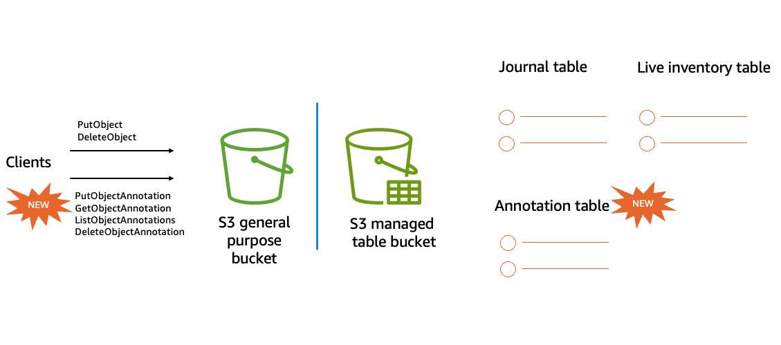

When you copy objects, you control whether annotations travel with them using the x-amz-object-annotation-directive header. Set this header to COPY (the default) to preserve annotations, or to EXCLUDE to omit them. For replication, Amazon S3 automatically replicates annotations associated with new objects to the destination bucket. When an object is deleted, its annotations are also deleted from the annotation table.

To query annotations at scale, surface them in S3 Metadata through the annotation table. You can also use natural language to search objects by their annotations using agents in Amazon SageMaker Unified Studio or an IDE with the S3 Tables MCP Server.

Materialized views

Materialized views are managed Iceberg tables in the AWS Glue Data Catalog that store precomputed query results. Unlike regular views, materialized views persist their results to storage and can be incrementally refreshed as underlying data changes. This means complex aggregations and joins that would normally take minutes can return in seconds.

In AWS Glue, you create materialized views using standard Spark SQL (refer to Using materialized views with AWS Glue for the configuration). The Data Catalog handles change detection, refresh scheduling, and compute infrastructure automatically.

In the fuel receipt scenario that follows, materialized views reduced query time by up to 93% and data scanned by 99%, turning a 19-second full-JSON scan into a 1.4-second lookup over 6 MB of precomputed results.

Walkthrough overview

The solution in this post consists of the following workflow:

Store scanned fuel receipts from fleet vehicles in a general purpose bucket to Amazon S3.
Use Amazon Bedrock Data Automation to extract structured data from each receipt and store the results as annotations.
Let S3 Metadata capture annotation data into a queryable Iceberg table.
Create materialized views in AWS Glue of pre-aggregated fuel spending data for fast fleet analytics.
Query the materialized views, powering dashboards for fuel cost breakdowns, vendor analysis, and geographic trends.

The following diagram shows the data flow.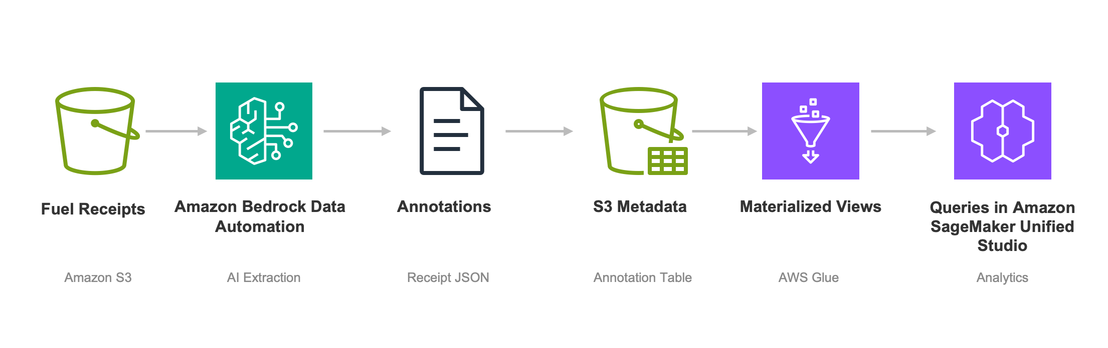 Solution data flow This pattern applies across industries and document types, including the following:

Financial services – Loan applications, invoices, tax forms, and KYC documents carry extracted fields as queryable annotations, enabling compliance audits and reconciliation.
Insurance – Claims forms, policy documents, and adjuster reports retain structured extraction results and classification metadata, streamlining claims processing and fraud detection.
Healthcare and life sciences – Patient intake forms, lab results, clinical trial documents, and medical imaging reports store normalized data with the source, supporting regulatory reporting and record reconciliation.
Media and entertainment – Technical metadata, rights information, content ratings, and AI-generated labels attach directly to media assets for catalog discovery and distribution workflows.
Manufacturing and supply chain – Inspection reports, certificates of conformance, sensor data, operational reports, and shipping documents carry structured quality and logistics data for traceability queries.

Prerequisites

To implement this solution, you must have the following:

An AWS account with S3, SageMaker Unified Studio, and AWS Glue access
An S3 general purpose bucket. (For this walkthrough, we use amzn-s3-demo-bucket. Replace with your own bucket). This walkthrough uses us-east-2; replace with your preferred AWS Region.
An S3 table bucket for storing materialized views.
S3 Tables integration with AWS analytics services enabled for your table bucket.
The latest version of the AWS Command Line Interface (AWS CLI).
AWS Lake Formation permissions configured for your S3 Tables.

Upload fuel receipt images

First, let’s upload scanned fuel receipts to our bucket. In a real scenario, these would be receipt photos captured by fleet drivers using a mobile app or scanned at fuel stations. For this walkthrough, we use 1,000 receipts for simplicity. The performance measurements later in this post were conducted on a 10 million receipt dataset to demonstrate behavior at scale.

Attach extraction results as annotations

After processing each receipt image through Amazon Bedrock Data Automation, we attach the structured extraction results as an annotation. Amazon Bedrock Data Automation extracts vendor name, location, fuel products, volumes, prices, payment method, and totals from each receipt. For instructions for setting up Amazon Bedrock Data Automation to extract metadata from documents, refer to Scalable intelligent document processing using Amazon Bedrock Data Automation.

The following code is a representative annotation payload for a single fuel receipt:

cat > /tmp/annotation.json << 'EOF'
{
  "file_name": "receipt_000001.jpg",
  "date": "04/28/2026",
  "vendor_name": "QuikTrip",
  "location": "1425 Highway 85 N, Fayetteville, GA 30214",
  "phone": "770-555-0142",
  "odometer": "104562",
  "payment_mode": "Visa",
  "product_1": "Diesel",
  "unit_of_measure_1": "Gallons",
  "volume_1": "87.432",
  "price_per_unit_1": "3.899",
  "product_2": "DEF",
  "unit_of_measure_2": "Gallons",
  "volume_2": "4.5",
  "price_per_unit_2": "2.799",
  "tax": "4.12",
  "total_amount": "353.56"
}
EOF

# Attach the annotation
aws s3api put-object-annotation \
  --bucket amzn-s3-demo-bucket \
  --key "receipts/receipt_000001.jpg" \
  --annotation-name fuel_receipt \
  --annotation-payload /tmp/annotation.json \
  --region us-east-2

# Verify it was attached
aws s3api list-object-annotations \
  --bucket amzn-s3-demo-bucket \
  --key "receipts/receipt_000001.jpg" \
  --region us-east-2

The list-object-annotations response confirms the annotation exists:

{
    "Annotations": [
        {
            "AnnotationName": "fuel_receipt",
            "LastModified": "2026-05-18T16:46:18+00:00",
            "ETag": "\"60e1b76770daa0ca39563f03ecc882e2\"",
            "ChecksumAlgorithm": [
                "CRC64NVME"
            ],
            "Size": 496
        }
    ],
    "Bucket": "amzn-s3-demo-bucket",
    "Key": "receipts/receipt_000001.jpg",
    "AnnotationCount": 1
}

In practice, you’d attach annotations programmatically as part of your receipt processing pipeline; call Amazon Bedrock Data Automation to extract the receipt data, then use the AWS SDK to attach the results as an annotation.

Enable annotation metadata table

To query annotations at scale, enable S3 Metadata with the annotation table configuration on your bucket using the CreateBucketMetadataConfiguration API.

1. Create an AWS Identity and Access Management (IAM) role with a trust policy that allows S3 Metadata to assume it:

{
  "Version": "2012-10-17",
  "Statement": [
    {
      "Effect": "Allow",
      "Principal": {
        "Service": "metadata.s3.amazonaws.com"
      },
      "Action": "sts:AssumeRole",
      "Condition": {
        "StringEquals": {
          "aws:SourceAccount": "111122223333"
        },
        "ArnLike": {
          "aws:SourceArn": "arn:aws:s3:::amzn-s3-demo-bucket"
        }
      }
    }
  ]
}

Note the Amazon Resource Name (ARN) of the role; you will need it later to enable the metadata configuration.

2. Create and attach the permissions policy:

{ 
   "Version": "2012-10-17", 
   "Statement": [ 
    { 
     "Effect": "Allow", 
     "Action": [ 
      "s3:GetObjectAnnotation", 
      "s3:GetObjectVersionAnnotation", 
      "s3:ListBucket", 
      "s3:ListBucketVersions" 
     ], 
     "Resource": [ 
      "arn:aws:s3:::amzn-s3-demo-bucket", 
      "arn:aws:s3:::amzn-s3-demo-bucket/*" 
     ] 
    } 
   ] 
  }

The caller enabling the metadata configuration also needs iam:PassRole permission for this role with the condition "iam:PassedToService": "metadata.s3.amazonaws.com". For full details on caller permissions, see Setting up permissions for configuring metadata tables.

3. Enable the annotation metadata table:

aws s3api create-bucket-metadata-configuration \
  --bucket amzn-s3-demo-bucket \
  --region us-east-2 \
  --metadata-configuration '{
    "JournalTableConfiguration": {
      "RecordExpiration": {"Expiration": "DISABLED"}
    },
    "InventoryTableConfiguration": {"ConfigurationState": "DISABLED"},
    "AnnotationTableConfiguration": {"ConfigurationState": "ENABLED", "Role": "${role_arn}"}
  }'

After you enable the annotation table, Amazon S3 automatically populates the table as annotations are created, updated, or deleted. The table follows the naming convention aws-s3.b_<bucket-name>.annotation and includes columns for the object key, annotation name, content (text_value), timestamps, and more. For details about the schema, refer to S3 Metadata annotation table schema.

The annotation content is stored in the text_value column. It contains the complete JSON annotation payload as a String, which means you can parse and aggregate annotation content directly in SQL.

Query annotation table in SageMaker Unified Studio

With the annotation table populated, let’s query it using the SQL editor in SageMaker Unified Studio. Select the S3 Tables catalog and the annotation table namespace in the editor, then run queries using the json_extract_scalar function to extract fields from the text_value column. The following queries assume you have selected the S3 Tables catalog and annotation table namespace in the SQL editor.

Explore data

First, let’s preview the annotation table and extract some key fields:

SELECT
  object_key,
  json_extract_scalar(text_value, '$.vendor_name') AS vendor,
  json_extract_scalar(text_value, '$.product_1') AS fuel_type,
  json_extract_scalar(text_value, '$.location') AS location,
  CAST(json_extract_scalar(text_value, '$.total_amount') AS DOUBLE) AS total_amount
FROM annotation
LIMIT 10

Run analytical queries against raw JSON

Now let’s run some typical fleet analytics queries. Each query must parse the full JSON payload for every row; with 10,000,000 receipts, that means parsing JSON on every scan.

Vendor distribution:

-- Count how many receipts each vendor has, then calculate percentage of total receipts it represent?

SELECT
   json_extract_scalar(text_value, '$.vendor_name') AS vendor,
   COUNT(*) AS cnt,
   ROUND(COUNT(*) * 100.0 / SUM(COUNT(*)) OVER(), 1) AS pct
 FROM annotation
 GROUP BY json_extract_scalar(text_value, '$.vendor_name')
 ORDER BY cnt DESC

Fuel type distribution:

-- What fuel products is the fleet purchasing?

SELECT
  json_extract_scalar(text_value, '$.product_1') AS fuel_type,
  COUNT(*) AS fill_count,
  ROUND(SUM(CAST(json_extract_scalar(text_value, '$.volume_1') AS DOUBLE)), 2) AS total_gallons,
  ROUND(AVG(CAST(json_extract_scalar(text_value, '$.price_per_unit_1') AS DOUBLE)), 3) AS avg_price_per_gallon
FROM annotation
WHERE name = 'fuel_receipt'
GROUP BY json_extract_scalar(text_value, '$.product_1')
ORDER BY total_gallons DESC

Payment mode analysis:

-- How are drivers paying for fuel?

SELECT
   json_extract_scalar(text_value, '$.payment_mode') AS payment_mode,
   COUNT(*) AS cnt,
   ROUND(AVG(CAST(json_extract_scalar(text_value, '$.total_amount') AS DOUBLE)), 2) AS avg_total,
   ROUND(SUM(CAST(json_extract_scalar(text_value, '$.total_amount') AS DOUBLE)), 2) AS sum_total
 FROM annotation
 GROUP BY json_extract_scalar(text_value, '$.payment_mode')
 ORDER BY cnt DESC

Each query scans the entire text_value column and parses JSON for every row. In our testing with 10 million annotations, the vendor distribution query took 19.2 seconds and scanned 525 MB of raw JSON data.

Accelerate queries with materialized views

You can use materialized views to simplify data transformation pipelines and accelerate query performance for complex queries. Instead of parsing JSON on every query, we pre-extract the fields we need into flat, typed Iceberg columns; one time. Subsequent queries read compact columnar data instead of scanning raw JSON.

Unlike regular views, they persist results in customer managed S3 Tables buckets and can be incrementally refreshed as the underlying annotation table changes. The Data Catalog handles change detection, refresh scheduling, and compute infrastructure automatically. For more information, refer to Introducing Apache Iceberg materialized views in AWS Glue Data Catalog.

Configure AWS Glue job

Before creating materialized views, configure your AWS Glue ETL job (version 5.1+) with the required Spark settings. You need two catalogs:

s3t_source – Reads from the S3 Metadata annotation table
s3t_catalog – Writes materialized views to your S3 Tables bucket

Refer to Configuring Spark to use materialized views for full configuration details.

If your bucket name contains hyphens, add spark.sql.catalog.<catalogName>.glue.skip-name-validation=true to your catalog configuration and use backticks around the namespace (for example, `b_amzn-s3-demo-bucket`) in your SQL statements.

Create materialized views

We create two views: an aggregated summary for dashboard queries, and a flattened detail table for drill-down and audit queries.

Fuel spending summary by vendor, fuel type, and payment (aggregated):

spark.sql("""
CREATE MATERIALIZED VIEW s3t_catalog.fuel_analytics.fuel_summary_by_vendor
SCHEDULE REFRESH EVERY 1 HOUR
AS
SELECT
  get_json_object(text_value, '$.vendor_name') AS vendor_name,
  get_json_object(text_value, '$.product_1') AS fuel_type,
  get_json_object(text_value, '$.payment_mode') AS payment_mode,
  COUNT(*) AS transaction_count,
  SUM(CAST(get_json_object(text_value, '$.total_amount') AS DOUBLE)) AS total_spend,
  SUM(CAST(get_json_object(text_value, '$.volume_1') AS DOUBLE)) AS total_gallons,
  AVG(CAST(get_json_object(text_value, '$.price_per_unit_1') AS DOUBLE)) AS avg_price_per_gallon,
  SUM(CAST(get_json_object(text_value, '$.tax') AS DOUBLE)) AS total_tax,
  MIN(last_modified_date) AS earliest_transaction,
  MAX(last_modified_date) AS latest_transaction
FROM s3t_source.`b_amzn-s3-demo-bucket`.annotation
WHERE name = 'fuel_receipt'
GROUP BY
  get_json_object(text_value, '$.vendor_name'),
  get_json_object(text_value, '$.product_1'),
  get_json_object(text_value, '$.payment_mode')
""")

Fuel receipt detail (flattened):

spark.sql("""
CREATE MATERIALIZED VIEW s3t_catalog.fuel_analytics.fuel_receipt_detail
SCHEDULE REFRESH EVERY 1 HOUR
AS
SELECT
  object_key,
  get_json_object(text_value, '$.file_name') AS file_name,
  get_json_object(text_value, '$.date') AS receipt_date,
  get_json_object(text_value, '$.vendor_name') AS vendor_name,
  get_json_object(text_value, '$.location') AS location,
  get_json_object(text_value, '$.odometer') AS odometer,
  get_json_object(text_value, '$.payment_mode') AS payment_mode,
  get_json_object(text_value, '$.product_1') AS fuel_type,
  CAST(get_json_object(text_value, '$.volume_1') AS DOUBLE) AS volume_gallons,
  CAST(get_json_object(text_value, '$.price_per_unit_1') AS DOUBLE) AS price_per_gallon,
  get_json_object(text_value, '$.product_2') AS secondary_product,
  CAST(get_json_object(text_value, '$.volume_2') AS DOUBLE) AS secondary_volume,
  CAST(get_json_object(text_value, '$.price_per_unit_2') AS DOUBLE) AS secondary_price,
  CAST(get_json_object(text_value, '$.tax') AS DOUBLE) AS tax,
  CAST(get_json_object(text_value, '$.total_amount') AS DOUBLE) AS total_amount,
  last_modified_date
FROM s3t_source.`b_amzn-s3-demo-bucket`.annotation
WHERE name = 'fuel_receipt'
""")

The SCHEDULE REFRESH EVERY 1 HOUR clause sets the minimum refresh interval. The Data Catalog detects changes in the source annotation table and triggers incremental refreshes automatically. You can also trigger a manual refresh at your desired time.

Verify materialized view

Both views are stored as Iceberg tables in your S3 Tables bucket, benefiting from automatic compaction and optimization. Verify the status with the following commands:

aws glue get-table \
    --catalog-id "111122223333:s3tablescatalog/my-table-bucket" \
    --database-name "fuel_analytics" \
    --name "fuel_summary_by_vendor" \
    --query "Table.{IsMaterializedView:IsMaterializedView, RefreshSeconds:ViewDefinition.RefreshSeconds, Source:ViewDefinition.SubObjects[0], IsStale:ViewDefinition.Representations[0].IsStale}"
{
    "IsMaterializedView": true,
    "RefreshSeconds": 3600,
    "Source": "arn:aws:glue:us-east-2:111122223333:table/s3tablescatalog/aws-s3/b_amzn-s3-demo-bucket/annotation",
    "IsStale": false
}

Query materialized views

Use the following commands to query the materialized views.

Vendor distribution (from detail view):

SELECT
   vendor_name AS vendor,
   COUNT(*) AS cnt,
   ROUND(COUNT(*) * 100.0 / SUM(COUNT(*)) OVER(), 1) AS pct
 FROM fuel_receipt_detail
 GROUP BY vendor_name
 ORDER BY cnt DESC

Fuel type distribution (from summary view):

SELECT
  fuel_type,
  SUM(transaction_count) AS fill_count,
  ROUND(SUM(total_gallons), 2) AS total_gallons,
  ROUND(SUM(total_spend) / SUM(total_gallons), 3) AS avg_price_per_gallon
FROM fuel_summary_by_vendor
GROUP BY fuel_type
ORDER BY total_gallons DESC

Payment mode analysis (from summary view):

SELECT
   payment_mode,
   COUNT(*) AS cnt,
   ROUND(AVG(total_amount), 2) AS avg_total,
   ROUND(SUM(total_amount), 2) AS sum_total
 FROM fuel_receipt_detail
 GROUP BY payment_mode
 ORDER BY cnt DESC

Price comparison across vendors (from detail view):

SELECT
  vendor_name,
  fuel_type,
  COUNT(*) AS transactions,
  ROUND(AVG(price_per_gallon), 3) AS avg_price,
  ROUND(MIN(price_per_gallon), 3) AS min_price,
  ROUND(MAX(price_per_gallon), 3) AS max_price
FROM fuel_receipt_detail
WHERE fuel_type = 'Diesel'
GROUP BY vendor_name, fuel_type
ORDER BY avg_price ASC
LIMIT 20

Monthly fuel cost trend (from detail view):

SELECT
  SUBSTR(receipt_date, 1, 2) AS month,
  COUNT(*) AS transactions,
  ROUND(SUM(total_amount), 2) AS monthly_spend,
  ROUND(SUM(volume_gallons), 2) AS monthly_gallons,
  ROUND(AVG(price_per_gallon), 3) AS avg_price
FROM fuel_receipt_detail
GROUP BY SUBSTR(receipt_date, 1, 2)
ORDER BY month

During our testing with 10 million annotations, the vendor distribution query completed in 1.4 seconds scanning just 6 MB of data with the materialized view, compared to 19.2 seconds scanning 525 MB when parsing raw JSON; a 93% reduction in query time and 99% less data scanned. Similarly, payment mode analysis dropped from 9.1 seconds (525 MB scanned) to 1.4 seconds (35 MB scanned); an 85% improvement in query time and 93% less data scanned.

Refresh materialized views

The materialized views refresh automatically every hour. You can also trigger a manual refresh:

spark.sql("REFRESH MATERIALIZED VIEW fuel_summary_by_vendor FULL")
spark.sql("REFRESH MATERIALIZED VIEW fuel_receipt_detail FULL")

Incremental refresh is particularly efficient for annotation tables because S3 Metadata captures changes as they happen; the refresh only needs to process new or modified annotations since the last refresh.

Cost considerations

Consider the following costs when using this solution:

Annotation storage – Annotation storage is charged at S3 Standard rates, regardless of the storage class of the associated parent object. You also pay standard S3 PUT and GET request rates for adding and retrieving annotations.
Annotation table storage – If you enable S3 Metadata tables, you pay additional charges for your annotation table, stored in an AWS managed S3 Tables bucket.
Materialized view storage – Materialized views are stored as Iceberg tables in your S3 Tables bucket, benefiting from automatic compaction and storage optimization. Storage costs depend on the size of the pre-aggregated results, which are typically much smaller than the source data.
Refresh compute – The Data Catalog uses managed Spark compute for refresh operations. Incremental refreshes minimize compute costs by processing only changed data.

Running many queries amplifies the benefits of faster response times and reduced data scanned, lowering compute costs and potentially offsetting the cost of maintaining materialized views.

Cleaning up

To remove the resources created in this walkthrough, use the following commands:

# Drop materialized views
spark.sql("DROP MATERIALIZED VIEW IF EXISTS fuel_summary_by_vendor")
spark.sql("DROP MATERIALIZED VIEW IF EXISTS fuel_receipt_detail")

# Delete the metadata configuration
aws s3api delete-bucket-metadata-configuration \
  --bucket amzn-s3-demo-bucket \
  --region us-east-2

# Delete annotations from objects
aws s3api delete-object-annotation \
  --bucket amzn-s3-demo-bucket \
  --key "receipts/receipt_000001.jpg" \
  --annotation-name fuel_receipt \
  --region us-east-2

Empty and delete the S3 bucket only if you had created to test this blog. Be careful with this step as if a bucket is deleted, it can’t be restored by AWS.

Delete the S3 Metadata tables:

aws s3tables delete-table \
--table-bucket-arn arn:aws:s3tables:us-east-2:111122223333:bucket/aws-s3 \
--namespace b_amzn-s3-demo-bucket \
--name journal \
--region us-east-2

aws s3tables delete-table \
--table-bucket-arn arn:aws:s3tables:us-east-2:111122223333:bucket/aws-s3 \
--namespace b_amzn-s3-demo-bucket \
--name annotation \
--region us-east-2

Conclusion

With S3 annotations, you can attach rich metadata to your S3 objects, giving AI agents and analytics tools the context they need to find and use the right data without building or maintaining separate metadata systems. In this post, we showed how a fleet fuel management workflow can extract structured data from fuel receipts, store the results as S3 annotations, and then query them at scale through materialized views in SageMaker Unified Studio.

The core pattern is straightforward: extract metadata from your documents using the tool that fits your workflow, store the results as annotations on the source object, and query them through S3 Metadata tables. The extraction layer can be Amazon Bedrock Data Automation, Amazon Textract, a custom machine learning (ML) model, or a third-party processor; S3 annotations is agnostic to how the metadata was produced. What matters is that once stored, your structured data lives with the source object, stays current through its lifecycle, and becomes queryable at scale without ETL pipelines or custom infrastructure.

To learn more, refer to Annotating your objects, Working with object metadata, and the Amazon SageMaker Unified Studio user guide. For pricing information, visit the Amazon S3 pricing page.

AWS Storage Blog