Building a Predictive Maintenance Solution Using AWS AutoML and No-Code Tools

By Volodymyr Koliadin, Sr. Data Scientist – Grid Dynamics
By Andriy Drebot, Data Scientist – Grid Dynamics
By Kavita Mahajan, Sr. Solutions Architect – AWS

Grid Dynamics

Industrial machine, equipment, and vehicle operators are often faced with the challenge of minimizing maintenance costs under strict constraints related to safety, equipment downtime, and other service-level agreements (SLAs).

Over-sufficient or preventive maintenance leads to resource underutilization and excessive maintenance costs. Meanwhile, under-sufficient or reactive maintenance can result in equipment downtime, safety risks, and revenue loss due to defects and failure propagation.

This challenge can be addressed by using predictive maintenance techniques that optimize the maintenance schedule and provide real-time insight on equipment condition and dynamics.

In this post, we describe how equipment operators can build a predictive maintenance solution using AutoML and no-code tools powered by Amazon Web Services (AWS).

This type of solution delivers significant gains to large-scale industrial systems and mission-critical applications where costs associated with machine failure or unplanned downtime can be high.

The design of this solution is based on the experience of Grid Dynamics with manufacturing clients. An engineering services company known for transformative cloud solutions, Grid Dynamics is an AWS Advanced Tier Services Partner with Competencies in DevOps and Data and Analytics.

Remaining Useful Life: An Actionable Metric

One of the most common tools for maintenance schedule optimization is a model that estimates the remaining useful life (RUL) of machines or equipment.

The RUL of a unit of equipment is the duration of time between its current operation and eventual failure. RUL can be estimated in time units such as hours or days, but it can also be estimated in discrete or continuous units of measurement. For example, the RUL of a cartridge for laser printers is expressed in the number of printed pages, while the RUL of an electric accumulator battery is expressed in charge-discharge cycles.

RUL estimates can be used to plan maintenance operations in ways that balance resource usage and failure risks.

The RUL is usually estimated using machine learning (ML) methods based on current equipment conditions. This generally requires creating a dataset that includes historical Internet of Things (IoT) metrics collected from sensors and failure events, developing an RUL model, and scoring the ongoing condition snapshots.

Solution Overview

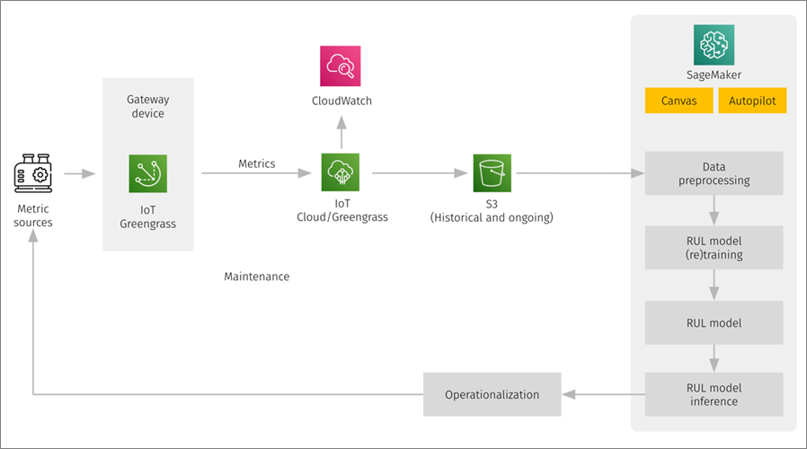
The high-level solution overview includes integrations with IoT metric sources that can be implemented using AWS IoT Greengrass, metrics journaling to Amazon Simple Storage Service (Amazon S3) or other storage, data preprocessing, RUL model training, model inference, and the operationalization of estimation results.

Figure 1 – High-level solution architecture.

RUL Model Design

There are several approaches to RUL prediction, and we use the direct regression-based approach to predict RUL as a numeric value expressed in the units of time remaining until equipment failure.

The initial data for the prediction (features) are the readings from different sensors describing the current state of the system. We also include the “time” variable into the feature set that characterizes the “age” of the system.

The target variable is the numerical value of the RUL expressed in time units. The goal of training the regression model is to obtain such predictions of the target from features that convey some predefined measure of the error as minimal.

Figure 2 – Design of the model for RUL prediction.

Quality Criteria and Evaluation Metrics

In regression analysis, the most frequently used measures of the aggregated error are Root Mean Square Error (RMSE) and Mean Absolute Error (MAE).

We strongly prefer using RMSE for the prediction of RUL because it’s less tolerant than MAE when it comes to large prediction errors. Large prediction errors leading to a gross overestimation of RUL may incur too high a cost associated with an unpredicted failure.

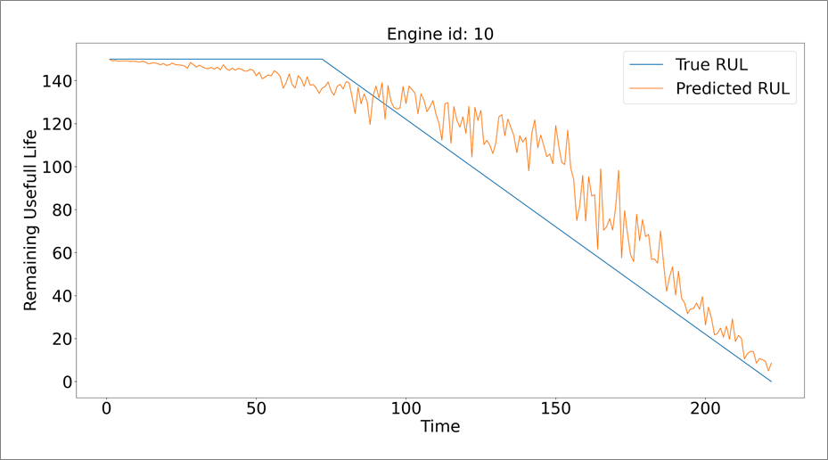
Besides the value of the aggregated error, like RMSE, it’s useful to check the individual predictions of the trained model for the test dataset—that is, a subset of the initial data not used for training the model. When such predictions are visualized along with true RUL values as a function of time, visual plot inspection can reveal a lot about model quality.

Dataset for Prototyping

To implement a prototype of the RUL model, we use a publicly available dataset known as NASA Turbofan Jet Engine Data Set. This dataset is often used for research and ML competitions.

The dataset includes degradation trajectories of 100 turbofan engines obtained from a simulator. Here, we explore only one of the four sub-datasets included, namely the training part of the dataset: FD001.

The time variable is expressed in discrete units, or cycles. The last point of the trajectory for each engine is the last cycle before the engine fails. We excluded some columns of the initial 26 columns; namely three columns with operational conditions (known to be constant for this set), as well as readings of several sensors known to be non-informative.

We also added a column (“rul”) with RUL values—that is, the number of cycles before the engine’s failure, clipped by upper value 150. The maximal RUL value 150 is used because exploratory data analysis shows that higher values of the remaining life are associated with too little degradation.

As such, the dataset is represented by a single table with the following columns:

(1) engine_id
(2) time
(3) rul
14 columns with the selected sensors’ readings named as sensor_XX, where XX is the number of the sensor in the initial dataset.

The layout of the dataset is shown here:

Figure 3 – Pre-processed NASA Turbofan Jet Engine Data Set.

RUL Model Implementation Using AutoML Tools

The traditional approach to developing a machine learning model requires performing a number of steps, such as:

Data preprocessing
Model design
Feature selection and engineering
Model training, validation, and fine-tuning
Model interpretation
Production deployment and monitoring.

Many of these steps can be executed only by ML and data science experts. AutoML allows us to automate the traditional workflow and replace it with steps that can be taken by non-experts in ML and data science.

In the following sections, we show how to implement two variants of this approach using different Amazon SageMaker components. For each variant, we build a complete pipeline that includes all of the necessary steps, starting with the initial data preprocessing to obtain meaningful RUL predictions.

Implementation Using Amazon SageMaker Canvas

In this section, we implement the RUL model using the no-code tool Amazon SageMaker Canvas. At a high level, the workflow consists of two major stages: model creation/deployment and inference.

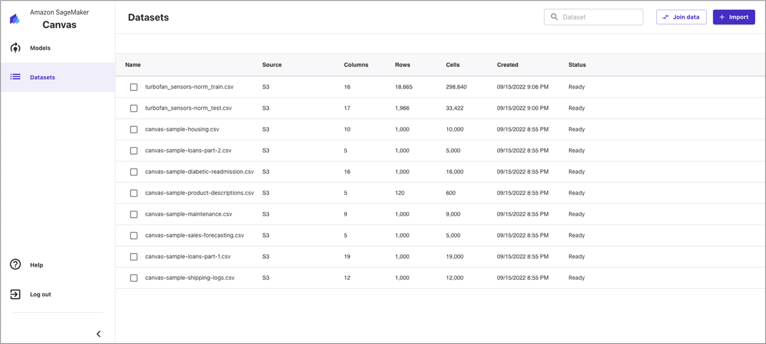
Import the Data to AWS Canvas

Before using Canvas, we need to upload our data to an Amazon S3 bucket. There is also an option to upload data just using a browser, or connecting Amazon Redshift or Snowflake.

Figure 4 – Browsing the available datasets in Canvas.

After we click the Import button, we are ready to import our data. Then we select our data from the list of files.

Create the Model

Now, we can create the model. Building the model takes only two steps:

Select: We prepare our dataset for training by selecting the relevant dataset from the list of the file we just uploaded.

Figure 5 – Selecting a dataset for model training.

Build: In this step, we choose our target column and the type of prediction task. In our case, it’s the column for “rul” and “Numeric” prediction (basically, Regression). We then choose how to build our model, either a quick vs. standard build. For the sake of this explainer, we choose a quick build. It’s worth noting we can select features for training by simply marking them.

Figure 6 – Specifying features and target variables for model training.

It’s important to bear in mind that a major part of AutoML magic has taken place under the hood at this step. A large number of models have been trained and evaluated on the data we uploaded, and then various sets of hyperparameters of the models have been tried and the best model has been selected for future use and deployed to the endpoint.

Analyze the Feature Importance and Performance

Once the optimal model has been selected, we try to gain some insight into its performance. Typically, we’d want to know some aggregated prediction error that might be expected from these sorts of data. RMSE is reported below.

We are also interested in discerning how important particular features are for the final prediction, and how any particular feature affects the predicted value. We can do this sort of analysis by pressing the Data visualizer button.

Figure 7 – Exploratory data analysis.

At this step, we check the model performance. In the case of Numeric Prediction, we have reported the RMSE metric. We can also check the feature importance and plot that describes how each feature influences our target metric.

Figure 8 – Feature importance analysis.

Making RUL Predictions

At this step, we are using our trained model to make predictions. There are two methods for prediction: batch prediction and single prediction.

In batch prediction, we use an uploaded dataset in order to predict our target variable for each row in the dataset. Once the prediction is ready we can preview or download the file.

Figure 9 – Batch prediction on a test dataset.

If we wish to look at an individual prediction (for one row in our dataset), we simply input feature values manually and create an individual prediction. This option could be useful for experimentation and manual testing of the model. We simply input the values of the features that will provide us with the predictions.

Following that, we can change the value of a feature, obtain a new prediction, and compare it to the previously observed one.

Figure 10 – Feature importance analysis for an individual prediction.

Implementation Using Amazon SageMaker AutoPilot

Even though the web-based workflow described in the previous section might be satisfactory for engines, it’s not as suitable for other application areas.

When data arrives frequently, and automatically, the process of data processing should be automated. A web-based interface is hardly suitable in such situations. Therefore, we developed another workflow based on Amazon SageMaker Autopilot. This particular workflow is implemented using two Jupyter notebooks.

The first notebook (AutopilotMakeModel.ipynb) automates the steps described above, including model deployment. The second notebook (AutopilotPredictRUL.ipynb) automates the process of inference itself—that is, making predictions of RUL on the basis of new data. Both notebooks are accompanied by detailed comments, and, as such, both are self-explanatory.

Model Training and Evaluation

For the model creation, data from 90 randomly selected engines were uploaded to Amazon SageMaker Autopilot. We left the remaining 10 engines for our own independent testing. We found no statistically significant differences between the estimates of the RMSE self-reported by SageMaker Autopilot, and the value of RMSE obtained at our testing dataset with 10 engines.

The value of the RMSE is about 20 (cycles/flights). The magnitude of the aggregated error is about the same as that achieved by ML experts and published in solutions on Kaggle.

The model training step (or, technically, model fitting) is implemented by only two commands. First, we create an AutoML-object:

automl = AutoML(role=EXECUTION_ROLE,
   target_attribute_name='rul',  # the target variable we want to predict
   base_job_name=AUTO_ML_JOB_NAME,
   sagemaker_session=SESSION,
   max_candidates=MAX_NUMBER_OF_CANDIDATES,
   problem_type='Regression',
   job_objective={'MetricName': 'MSE'}
)

Then, we launch the process of model training (fitting) for the AutoML object with the following command:

automl.fit(
   inputs=DATA_LOCATION_S3_BUCKET,
   job_name=AUTO_ML_JOB_NAME,
   wait=True,  # wait the end of the training process
   logs=True,  # get the progress bar
)

After the command is finished, we know that SageMaker Autopilot has successfully created, trained, and optimized a bunch of models. We can explore the models and select the best option manually or automatically based on the RMSE metric.

To evaluate the quality of the model, we get the best model and output the values of several popular metrics estimated for the validation dataset generated automatically during the fitting process:

best_candidate = automl.best_candidate(job_name=AUTO_ML_JOB_NAME)
best_candidate['CandidateProperties']['CandidateMetrics']

--------------------------------------------------------------------------

[{'MetricName': 'MSE', 'Value': 466.4531555175781, 'Set': 'Validation'},
{'MetricName': 'MAE', 'Value': 16.749845504760742, 'Set': 'Validation'},
{'MetricName': 'R2', 'Value': 0.8132867217063904, 'Set': 'Validation'},
{'MetricName': 'RMSE', 'Value': 21.596208572387695, 'Set': 'Validation'}]

We can see from the output, for example, that the RMS-error of RUL prediction is about 21.6. We also see values of other metrics, like MSE, MAE, and R2. Typically, knowing such values allows us to make some judgment about the model and compare it to other models.

To better evaluate the model, we visualize the behavior of individual predictions for a particular engine:

The solid blue line in shows the true value of RUL (not known by the model).
The orange line shows the prediction of RUL produced by the model generated for different values of discrete time expressed in cycles/flights.

Figure 11 – Example of the predicted RUL trajectory.

Model Explainability: Feature Importance

A special type of model evaluation analyzes feature importance and other components. For many of Grid Dynamics’ clients, ML application areas are a mandatory step. Mere black-box-like models, which lack any explainability capabilities, are not satisfactory in many situations.

Fortunately, Amazon SageMaker Autopilot provides well-developed tools for these purposes. A single line of code allows us to identify the location of the file with the result of feature importance analysis:

best_candidate['CandidateProperties']['CandidateArtifactLocations']

It produces the following output with a path to the S3 folder where the results of feature importance analysis for the best model are located:

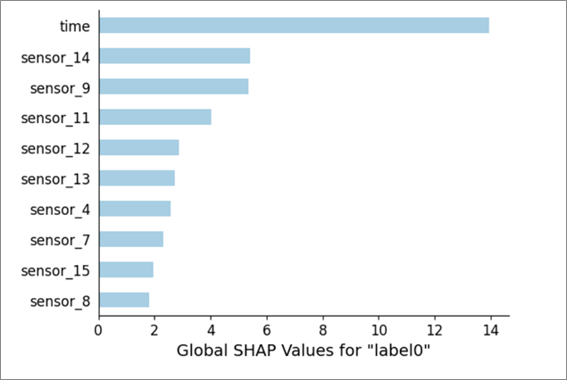
{'Explainability': 's3://sagemaker-us-east-1-283824160429/test-notebook-experiment-sm05/documentation/explainability/output',
…},

A PDF file in that folder shows the results of the feature importance analysis in an easily perceptible graphic form.

Figure 12 – Feature importance analysis using AutoPilot.

It’s easy to understand from the plot that the feature “time” is the most important one here, followed by the two features, “sensor_14” and “sensor_9”.

Model Deployment and Inference

When the optimal model has been trained and evaluated, we usually want to use it for inference—that is, for RUL prediction. There are at least two options to choose from.

First, we may rely on the batch prediction mode. In this case, we do not need to deploy the model; we simply specify a file with rows containing the observed feature values, run a batch-prediction job, and get the predictions of the RUL made by the model we trained above.

The second notebook contains a separate section (“Batch prediction”) that illustrates this process in detail.

For automated operations and real-time RUL estimation, it’s suitable to deploy the model first, and then use the corresponding endpoint for online predictions. The deployment itself is achieved by a single command that creates an endpoint with the given name (see section “Testing Our Endpoint” in the first notebook and section “Prediction Using Endpoint” in the second notebook).

automl.deploy(initial_instance_count=1, # how many machines are required
   instance_type='ml.m5.2xlarge', # machine type
   serializer=None,
   deserializer=None,
   candidate=None,  # if None, best candidate is used for deployment
   sagemaker_session=SESSION,
   endpoint_name=ENDPOINT_NAME,
   wait=True) # to see the progress below (deployment status)

Conclusion

Grid Dynamics developed two workflows for predicting remaining useful life (RUL) for various types of equipment. Both workflows cover the creation, deployment, and inference of the RUL model using Amazon SageMaker Canvas and SageMaker Autopilot.

In this post, we demonstrated the operation of both approaches using NASA Turbofan Jet Engine Data Set. The performance of the model created purely by the AutoML services is comparable to the published performance of models created by experts for the same dataset.

.

.

Grid Dynamics – AWS Partner Spotlight

Grid Dynamics is an AWS Advanced Tier Services Partner and engineering services company known for transformative cloud solutions.

Contact Grid Dynamics | Partner Overview | AWS Marketplace

AWS Partner Network (APN) Blog