Evaluate models with the Amazon Nova evaluation container using Amazon SageMaker AI

This blog post introduces the new Amazon Nova model evaluation features in Amazon SageMaker AI. This release adds custom metrics support, LLM-based preference testing, log probability capture, metadata analysis, and multi-node scaling for large evaluations.

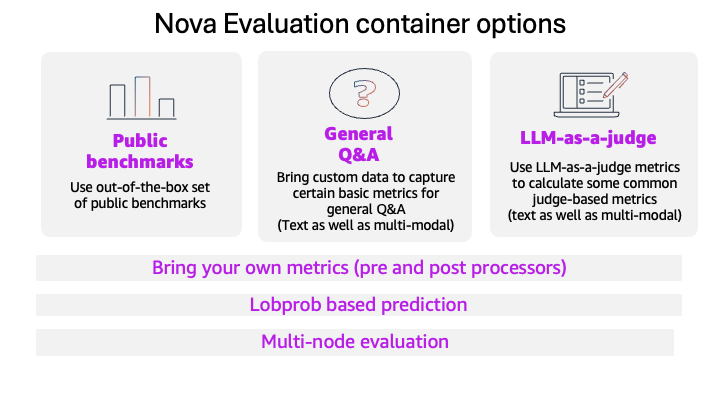
The new features include:

• Custom metrics use the bring your own metrics (BYOM) functions to control evaluation criteria for your use case.
• Nova LLM-as-a-Judge handles subjective evaluations through pairwise A/B comparisons, reporting win/tie/loss ratios and Bradley-Terry scores with explanations for each judgment.
• Token-level log probabilities reveal model confidence, useful for calibration and routing decisions.
• Metadata passthrough keeps per-row fields for analysis by customer segment, domain, difficulty, or priority level without extra processing.
• Multi-node execution distributes workloads while maintaining stable aggregation, scaling evaluation datasets from thousands to millions of examples.

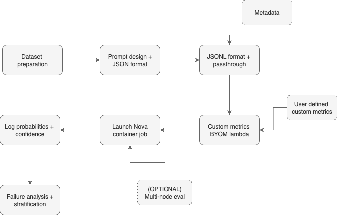
In SageMaker AI, teams can define model evaluations using JSONL files in Amazon Simple Storage Service (Amazon S3), then execute them as SageMaker training jobs with control over pre- and post-processing workflows with results delivered as structured JSONL with per-example and aggregated metrics and detailed metadata. Teams can then integrate results with analytics tools like Amazon Athena and AWS Glue, or directly route them into existing observability stacks, with consistent results.

The rest of this post introduces the new features and then demonstrates step-by-step how to set up evaluations, run judge experiments, capture and analyze log probabilities, use metadata for analysis, and configure multi-node runs in an IT support ticket classification example.

Features for model evaluation using Amazon SageMaker AI

When choosing which models to bring into production, proper evaluation methodologies require testing multiple models, including customized versions in SageMaker AI. To do so effectively, teams need identical test conditions passing the same prompts, metrics, and evaluation logic to different models. This makes sure score differences reflect model performance, not evaluation methods.

Amazon Nova models that are customized in SageMaker AI now inherit the full evaluation infrastructure as base models making it a fair comparison. Results land as structured JSONL in Amazon S3, ready for Athena queries or routing to your observability stack. Let’s discuss some of the new features available for model evaluation.

Bring your own metrics (BYOM)

Standard metrics might not always fit your specific requirements. Custom metrics features leverage AWS Lambda functions to handle data preprocessing, output post-processing, and metric calculation. For instance, a customer service bot needs empathy and brand consistency metrics; a medical assistant might require clinical accuracy measures. With custom metrics, you can test what matters for your domain.

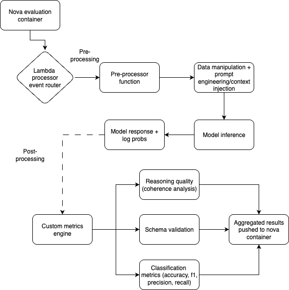
In this feature, pre- and post-processor functions are encapsulated in a Lambda function that is used to process data before inference to normalize formats or inject context and to then calculate your custom metrics using post-processing function after the model responds. Finally, the results are aggregated using your choice of min, max, average, or sum, thereby offering greater flexibility when different test examples carry varying importance.

Multimodal LLM-as-a-judge evaluation

LLM-as-a-judge automates preference testing for text as well as multimodal tasks using Amazon Nova LLM-as-a-Judge models for response comparison. The system implements pairwise evaluation: for each prompt, it compares baseline and challenger responses, running the comparison in both forward and backward passes to detect positional bias. The output includes Bradley-Terry probabilities (the likelihood one response is preferred over another) with bootstrap-sampled confidence intervals, giving statistical confidence in preference results.

Nova LLM-as-a-Judge models are purposefully customized for judging related evaluation tasks. Each judgment includes natural language rationales explaining why the judge preferred one response over other, helping with targeted improvements rather than blind optimization. Nova LLM-as-a-Judge evaluates complex reasoning tasks like support ticket classification, where nuanced understanding matters more than simple keyword matching.

The tie detection is equally valuable, identifying where models have reached parity. Combined with standard error metrics, you can determine whether performance differences are statistically meaningful or within noise margins; this is important when deciding if a model update justifies deployment.

Use log probability for model evaluation

Log probabilities show model confidence for each generated token, revealing insights into model uncertainty and prediction quality. Log probabilities support calibration studies, confidence routing, and hallucination detection beyond basic accuracy. Token-level confidence helps identify uncertain predictions for more reliable systems.

A Nova evaluation container with SageMaker AI model evaluation now captures token-level log probabilities during inference for uncertainty-aware evaluation workflows. The feature integrates with evaluation pipelines and provides the foundation for advanced diagnostic capabilities. You can correlate model confidence with actual performance, implement quality gates based on uncertainty thresholds, and detect potential issues before they impact production systems. Add log probability capture by adding the top_logprobs parameter to your evaluation configuration:

# Add log probability capture to your evaluation configuration
inference:
  max_new_tokens: 2048
  temperature: 0
  top_logprobs: 10  # Captures top 10 log probabilities per token

When combined with the metadata passthrough feature as discussed in the next section, log probabilities help with stratified confidence analysis across different data segments and use cases. This combination provides detailed insights into model behavior, so teams can understand not just where models fail, but why they fail and how confident they are in their predictions giving them more control over calibration.

Pass metadata information when using model evaluation

Custom datasets now support metadata fields when preparing the evaluation dataset. Metadata helps compare results across different models and datasets. The metadata field accepts any string for tagging and analysis with the input data and eval results. With the addition of the metadata field, the overall schema per data point in JSONL file becomes the following:

{
  "query": "(Required) String containing the question or instruction that needs an answer",
  "response": "(Required) String containing the expected model output",
  "system": "(Optional) String containing the system prompt that sets the behavior, role, or personality of the AI model before it processes the query",
  "metadata": "(Optional) String containing metadata associated with the entry for tagging purposes."
}

Enable multi-node evaluation

The evaluation container supports multi-node evaluation for faster processing. Set the replicas parameter to enable multi-node evaluation to a value greater than one.

Case study: IT support ticket classification assistant

The following case study demonstrates several of these new features using IT support ticket classification. In this use case, models classify tickets as hardware, software, network, or access issues while explaining their reasoning. This tests both accuracy and explanation quality, and shows custom metrics, metadata passthrough, log probability analysis, and multi-node scaling in practice.

Dataset overview

The support ticket classification dataset contains IT support tickets spanning different priority levels and technical domains, each with structured metadata for detailed analysis. Each evaluation example includes a support ticket query, the system context, a structured response containing the predicted category, the reasoning based on ticket content, and a natural language description. Amazon SageMaker Ground Truth responses include thoughtful explanations like Based on the error message mentioning network timeout and the user's description of intermittent connectivity, this appears to be a network infrastructure issue requiring escalation to the network team. The dataset includes metadata tags for difficulty level (easy/medium/hard based on technical complexity), priority (low/medium/high), and domain category, demonstrating how metadata passthrough works for stratified analysis without post-processing joins.

Prerequisites

Before you run the notebook, make sure the provisioned environment has the following:

1. An AWS account
2. AWS Identity and Access Management (IAM) permissions to create a Lambda function, the ability to run SageMaker training jobs within the associated AWS account in the previous step, and read and write permissions to an S3 bucket
3. A development environment with SageMaker Python SDK and the Nova custom evaluation SDK (nova_custom_evaluation_sdk)

Step 1: Prepare the prompt

For our support ticket classification task, we need to assess not only whether the model identifies the correct category, but also whether it provides coherent reasoning and adheres to structured output formats to have a complete overview required in production systems. For crafting the prompt, we are going to use Nova prompting best practices.

System prompt design: Starting with the system prompt, we establish the model’s role and expected behavior through a focused system prompt:

You are an IT support specialist. Analyze the support ticket and classify it accurately based on the issue description and technical details.

This prompt sets clear expectations: the model should act as a domain expert, base decisions on visual evidence, and prioritize accuracy. By framing the task as expert analysis rather than casual observation, we encourage more thoughtful, detailed responses.

Query structure: The query template requests both classification and justification:

# Query template requests classification and reasoning
"What category does this support ticket belong to? Provide your reasoning based on the issue description."

The explicit request for reasoning is important—it forces the model to articulate its decision-making process, helping with evaluation of explanation quality alongside classification accuracy. This mirrors real-world requirements where model decisions often need to be interpretable for stakeholders or regulatory compliance.

Structured response format: We define the expected output as JSON with three components:

{
  "class": "network_connectivity",
  "thought": "Based on the error message mentioning network timeout and intermittent connectivity issues, this appears to be a network infrastructure problem",
  "description": "Network connectivity issue requiring infrastructure team escalation"
}

This structure supports the three-dimensional evaluation strategy we will discuss later in this post:

• class field – Classification accuracy metrics (precision, recall, F1)
• thought field – Reasoning coherence evaluation
• description field – Natural language quality assessment

By defining the response as parseable JSON, we help with automated metric calculation through our custom Lambda functions while maintaining human-readable explanations for model decisions. This prompt architecture transforms evaluation from simple right/wrong classification into a complete assessment of model capabilities. Production AI systems need to be accurate, explainable, and reliable in their output formatting—and our prompt design explicitly tests all three dimensions. The structured format also facilitates the metadata-driven stratified analysis we’ll use in later steps, where we can correlate reasoning quality with confidence scores and difficulty levels across different breed categories.

Step 2: Prepare the dataset for evaluation with metadata

In this step, we’ll prepare our support ticket dataset with metadata support to help with stratified analysis across different categories and difficulty levels. The metadata passthrough feature keeps custom fields complete for detailed performance analysis without post-hoc joins. Let’s review an example dataset.

Dataset schema with metadata

For our support ticket classification evaluation, we’ll use the enhanced gen_qa format with structured metadata:

{
  "system": "You are a support ticket classification expert. Analyze the ticket content and classify it accurately based on the issue type, urgency, and department that should handle it.",
  "query": "My laptop won't turn on at all. I've tried holding the power button, checking the charger connection, but there's no response. The LED indicators aren't lighting up either.",
  "response": "{\"class\": \"Hardware_Critical\", \"thought\": \"Complete device failure with no power response indicates a critical hardware issue\", \"description\": \"Critical hardware failure requiring urgent IT support\"}",
  "metadata": "{\"category\": \"support_ticket_classification\", \"difficulty\": \"easy\", \"domain\": \"IT_support\", \"priority\": \"critical\"}"
}

Examine this further: how do we automatically generate structured metadata for each evaluation example? This metadata enrichment process analyzes the content to classify task types, assess difficulty levels, and identify domains, creating the foundation for stratified analysis in later steps. By embedding this contextual information directly into our dataset, we help the Nova evaluation pipeline keep these insights complete, so we can understand model performance across different segments without requiring complex post-processing joins.

import json
from typing import List, Dict

def load_sample_dataset(file_path: str = 'sample_text_eval_dataset.jsonl') -> List[Dict]:
    """Load the sample dataset with metadata"""
    dataset = []
    with open(file_path, 'r') as f:
        for line in f:
            dataset.append(json.loads(line))
    return dataset

Once our dataset is enriched with metadata, we need to export it in the JSONL format required by the Nova evaluation container.

The following export function formats our prepared examples with embedded metadata so that they are ready for the evaluation pipeline, maintaining the exact schema structure needed for the Amazon SageMaker processing workflow:

# Export for SageMaker Evaluation
def export_to_sagemaker_format(dataset: List[Dict], output_path: str = 'gen_qa.jsonl'):
    """Export dataset in format compatible with SageMaker """
    
    with open(output_path, 'w', encoding='utf-8') as f:
        for item in dataset:
            f.write(json.dumps(item, ensure_ascii=False) + '\n')
    
    print(f"Dataset exported: {len(dataset)} examples to {output_path}")

# Usage Example
dataset = load_sample_dataset('sample_text_eval_dataset.jsonl')
export_to_sagemaker_format(dataset)

Step 3: Prepare custom metrics to evaluate custom models

After preparing and verifying your data adheres to the required schema, the next important step is to develop evaluation metrics code to assess your custom model’s performance. Use Nova evaluation container and the bring your own metric (BYOM) workflow to control your model evaluation pipeline with custom metrics and data workflows.

Introduction to BYOM workflow

With the BYOM feature, you can tailor your model evaluation workflow to your specific needs with fully customizable pre-processing, post-processing, and metrics capabilities. BYOM gives you control over the evaluation process, helping you to fine-tune and improve your model’s performance metrics according to your project’s unique requirements.

Key tasks for this classification problem

1. Define tasks and metrics: In this use case, model evaluation requires three tasks:
   1. Class prediction accuracy: This will assess how accurately the model predicts the correct class for given inputs. For this we will use standard metrics such as accuracy, precision, recall, and F1 score to quantify performance.
   2. Schema adherence: Next, we also want to ensure that the model’s outputs conform to the specified schema. This step is important for maintaining consistency and compatibility with downstream applications. For this we will use validation techniques to verify that the output format matches the required schema.
   3. Thought process coherence: Next, we also want to evaluate the coherence and reasoning behind the model’s decisions. This involves analyzing the model’s thought process to help validate predictions are logically sound. Techniques such as attention mechanisms, interpretability tools, and model explanations can provide insights into the model’s decision-making process.

The BYOM feature for evaluating custom models requires building a Lambda function.

2. Configure a custom layer on your Lambda function. In the GitHub release, find and download the pre-built nova-custom-eval-layer.zip file.
3. Use the following command to upload the custom Lambda layer:

# Upload custom lambda layer for Nova evaluation
aws lambda publish-layer-version \
    --layer-name nova-custom-eval-layer \
    --zip-file fileb://nova-custom-eval-layer.zip \
    --compatible-runtimes python3.12 python3.11 python3.10 python3.9

4. Add the published layer and AWSLambdaPowertoolsPythonV3-python312-arm64 (or similar AWS layer based on Python version and runtime version compatibility) to your Lambda function to ensure all necessary dependencies are installed.
5. For development of the Lambda function, import two key dependencies: one for importing the preprocessor and postprocessor decorators and one to build the lambda_handler:

# Import required dependencies for Nova evaluation
from nova_custom_evaluation_sdk.processors.decorators import preprocess, postprocess
from nova_custom_evaluation_sdk.lambda_handler import build_lambda_handler

6. Add the preprocessor and postprocessor logic.
   1. Preprocessor logic: Implement functions that manipulate the data before it is passed to the inference server. This can include prompt manipulations or other data preprocessing steps. The pre-processor expects an event dictionary (dict), a sequence of key value pairs, as input:

      event = {
          "process_type": "preprocess",
          "data": {
              "system": < passed in system prompt>,
              "prompt": < passed in user prompt >,
              "gold": <expected_answer>
          }
      }

      Example:

      @preprocess
      def preprocessor(event: dict, context) -> dict:
          data = event.get('data', {})
          return {
              "statusCode": 200,
              "body": {
                  "system": data.get("system"),
                  "prompt": data.get("prompt", ""),
                  "gold": data.get("gold", "")
              }
          }

   2. Postprocessor logic: Implement functions that process the inference results. This can involve parsing fields, adding custom validations, or calculating specific metrics. The postprocessor expects an event dict as input which has this format:

      event = {
      "process_type": "postprocess",
      "data":{
          "prompt": < the input prompt >,
          "inference_output": < the output from inference on custom or base model >,
          "gold": < the expected output >
          }
      }

7. Define the Lambda handler, where you add the pre-processor and post-processor logics, before and after inference respectively.

   # Build Lambda handler
   lambda_handler = build_lambda_handler(
   preprocessor=preprocessor,
   postprocessor=postprocessor
   )
   

Step 4: Launch the evaluation job with custom metrics

Now that you have built your custom processors and encoded your evaluation metrics, you can choose a recipe and make necessary adjustments to make sure the previous BYOM logic gets executed. For this, first choose bring your own data recipes from the public repo, and make sure the following code changes are made.

1. Make sure that the processor key is added on to the recipe with correct details:

   # Processor configuration in recipe
   processor:
     lambda_arn: arn:aws:lambda:<region>:<account_id>:function:<name> 
     preprocessing:
       enabled: true
     postprocessing:
       enabled: true
     aggregation: average 

   • lambda-arn: The Amazon Resource Name (ARN) for a customer Lambda function that handles pre-processing and post-processing
   • preprocessing: Whether to add custom pre-processing operations
   • post-processing: Whether to add custom post-processing operations
   • aggregation: In-built aggregation function to choose from.
     min, max, average, or sum
2. Launch a training job with an evaluation container:

   # SageMaker training job configuration
   input_s3_uri = "s3://amzn-s3-demo-input-bucket/<jsonl_data_file>"  #  replace with your S3 URI and  <jsonl_data_file> with your actual file name
   output_s3_uri = "s3://amzn-s3-demo-input-bucket"  # Output results location
   instance_type = "ml.g5.12xlarge"  # Instance type for evaluation
   job_name = "nova-lite-support-ticket-class"
   recipe_path = "./class_pred_with_byom.yaml"  # Recipe configuration file
   image_uri = "708977205387.dkr.ecr.us-east-1.amazonaws.com/nova-evaluation-repo:SM-TJ-Eval-latest”   # Latest as of this post
   # Configure training input
   evalInput = TrainingInput(
       s3_data=input_s3_uri,
       distribution='FullyReplicated',
       s3_data_type='S3Prefix'
   )
   # Create and configure estimator
   estimator = PyTorch(
       output_path=output_s3_uri,
       base_job_name=job_name,
       role=role,
       instance_type=instance_type,
       training_recipe=recipe_path,
       sagemaker_session=sagemaker_session,
       image_uri=image_uri
   )
   # Launch evaluation job
   estimator.fit(
       inputs={"train": evalInput}

Step 5: Use metadata and log probabilities to calibrate the accuracy

You can also include log probability as an inference config variable to help conduct logit-based evaluations. For this we can pass top_logprobs under inference in the recipe:

top_logprobs indicates the number of most likely tokens to return at each token position each with an associated log probability. This value must be an integer from 0 to 20. Logprobs contain the considered output tokens and log probabilities of each output token returned in the content of message.

# Log probability configuration in inference settings
inference:
  max_new_tokens: 2048 
  top_k: -1 
  top_p: 1.0 
  temperature: 0
  top_logprobs: 10  # Number of most likely tokens to return (0-20)

Once the job runs successfully and you have the results, you can find the log probabilities under the field pred_logprobs. This field contains the considered output tokens and log probabilities of each output token returned in the content of message. You can now use the logits produced to do calibration for your classification task. The log probabilities of each output token can be useful for calibration, to adjust the predictions and treat these probabilities as confidence score.

Step 6: Failure analysis on low confidence prediction

After calibrating our model using metadata and log probabilities, we can now identify and analyze failure patterns in low-confidence predictions. This analysis helps us understand where our model struggles and guides targeted improvements.

Loading results with log probabilities

Now, let’s examine in detail how we combine the inference outputs with detailed log probability data from the Amazon Nova evaluation pipeline. This helps us perform confidence-aware failure analysis by merging the prediction results with token-level uncertainty information.

import pandas as pd
import json
import numpy as np
from sklearn.metrics import classification_report

def load_evaluation_results_with_logprobs(inference_output_path: str, details_parquet_path: str) -> pd.DataFrame:
    """Load inference results and merge with log probabilities"""
    
    # Load inference outputs
    results = []
    with open(inference_output_path, 'r') as f:
        for line in f:
            results.append(json.loads(line))
    
    # Load log probabilities from parquet
    details_df = pd.read_parquet(details_parquet_path)
    
    # Create results dataframe
    results_df = pd.DataFrame(results)
    
    # Add log probability data and calculate confidence
    if 'pred_lobprobs' in details_df.columns:
        results_df['pred_lobprobs'] = details_df['pred_lobprobs'].tolist()
        results_df['confidence'] = results_df['pred_lobprobs'].apply(calculate_confidence_score)
    
    # Calculate correctness and parse metadata
    results_df['is_correct'] = results_df.apply(calculate_correctness, axis=1)
    results_df['metadata_parsed'] = results_df['metadata'].apply(safe_parse_metadata)
    
    return results_df

Generate a confidence score from log probabilities by converting the logprobs to probabilities and using the score of the first token in the classification response. We only use the first token as we know subsequent tokens in the classification would align the class label. This step creates downstream quality gates in which we could route low confidence scores to human review, have a view into model uncertainty to validate if the model is “guessing,” preventing hallucinations from reaching users, and later enables stratified analysis.

def calculate_confidence_score(pred_logprobs_str, prediction_text="") -> tuple:
    """
    Calculate confidence score from log probabilities for the predicted class.
    
    Args:
        pred_logprobs_str (str): String representation of prediction logprobs (updated field name as of 10/23/25)
        prediction_text (str): The actual prediction text to extract class from
        
    Returns:
        tuple: (confidence, predicted_token, filtered_keys) - 
               confidence: The first token probability of the predicted class
               predicted_token: The predicted class name
               filtered_keys: List of tokens in the class name
    
    Note: Tokens may include SentencePiece prefix characters (▁) as of container update 10/23/25
    """
    if not pred_logprobs_str or pred_logprobs_str == '[]':
        return 0.0, "", []
    
    try:
        # Extract the predicted class from the prediction text
        predicted_class = ""
        if prediction_text:
            try:
                parsed = json.loads(prediction_text)
                predicted_class = str(parsed.get("class", "")).strip()
            except:
                predicted_class = ""
        
        if not predicted_class:
            return 0.0, "", []
        
        logprobs = ast.literal_eval(pred_logprobs_str)
        if not logprobs or len(logprobs) == 0:
            return 0.0, predicted_class, []
        
        # Build dictionary of all tokens and their probabilities
        token_probs = {}
        for token_prob_dict in logprobs[0]:
            if isinstance(token_prob_dict, dict) and token_prob_dict:
                max_key = max(token_prob_dict.items(), key=lambda x: x[1])[0]
                max_logprob = token_prob_dict[max_key]
                token_probs[max_key] = np.exp(max_logprob)
        
        # Find tokens that match the predicted class
        class_tokens = []
        class_probs = []
        
        # Split class name into potential tokens
        class_parts = re.split(r'[_\s]+', predicted_class)
        
        for token, prob in token_probs.items():
            # Strip SentencePiece prefix (▁) and other special characters for matching
            clean_token = re.sub(r'[^a-zA-Z0-9]', '', token)
            if clean_token:
                # Check if this token matches any part of the class name
                for part in class_parts:
                    if part and (clean_token.lower() == part.lower() or 
                                part.lower().startswith(clean_token.lower()) or
                                clean_token.lower().startswith(part.lower())):
                        class_tokens.append(clean_token)
                        class_probs.append(prob)
                        break
        
        # Use first token confidence (OpenAI's classification approach)
        if class_probs:
            confidence = float(class_probs[0])
        else:
            confidence = 0.0
        
        return confidence, predicted_class, class_tokens
    except Exception as e:
        print(f"Error processing log probs: {e}")
        return 0.0, "", []

Initial analysis

Next, we perform stratified failure analysis, which combines confidence scores with metadata categories to identify specific failure patterns. This multi-dimensional analysis reveals failure modes across different task types, difficulty levels, and domains. Stratified failure analysis systematically examines low-confidence predictions to identify specific patterns and root causes. It first filters predictions below the confidence threshold, then conducts multi-dimensional analysis across metadata categories to pinpoint where the model struggles most. We also analyze content patterns in failed predictions, looking for uncertainty language and categorizing error types (JSON format issues, length problems, or content errors) before generating insights that tell teams exactly what to fix.

def analyze_low_confidence_failures(results_df: pd.DataFrame, confidence_threshold: float = 0.7, quality_threshold: float = 0.3) -> dict:
    """Perform comprehensive failure analysis"""
    
    # Make a copy to avoid modifying original
    df = results_df.copy()
    
    # Helper to extract prediction text
    def get_prediction_text(row):
        pred = row['predictions']
        
        # Handle string representation of array: "['text']" 
        if isinstance(pred, str):
            try:
                pred_list = ast.literal_eval(pred)
                if isinstance(pred_list, list) and len(pred_list) > 0:
                    return str(pred_list[0]).strip()
            except:
                pass
        
        # Handle actual array
        if isinstance(pred, (list, np.ndarray)) and len(pred) > 0:
            return str(pred[0]).strip()
        
        return str(pred).strip()
    
    # Apply the function with both logprobs and prediction text
    confidence_results = df.apply(
        lambda row: calculate_confidence_score(row['pred_logprobs'], get_prediction_text(row)), 
        axis=1
    )
    df[['confidence', 'predicted_token', 'filtered_keys']] = pd.DataFrame(
        list(confidence_results), 
        index=df.index,
        columns=['confidence', 'predicted_token', 'filtered_keys']
    )
    
    df['quality_score'] = df['metrics'].apply(
        lambda x: ast.literal_eval(x).get('f1', 0) if x else 0
    )
    df['is_correct'] = df['quality_score'] >= quality_threshold
    
    # Analyze low confidence predictions
    low_conf_df = df[df['confidence'] < confidence_threshold]
    
    # Also identify high confidence but low quality (overconfident errors)
    overconfident_df = df[(df['confidence'] >= confidence_threshold) & 
                          (df['quality_score'] < quality_threshold)]
    
    analysis_results = {
        'summary': {
            'total_predictions': len(df),
            'low_confidence_count': len(low_conf_df),
            'low_confidence_rate': len(low_conf_df) / len(df) if len(df) > 0 else 0,
            'overconfident_errors': len(overconfident_df),
            'overconfident_rate': len(overconfident_df) / len(df) if len(df) > 0 else 0,
            'avg_confidence': df['confidence'].mean(),
            'avg_quality': df['quality_score'].mean(),
            'overall_accuracy': df['is_correct'].mean()
        },
        'low_confidence_examples': [],
        'overconfident_examples': []
    }
    
    # Low confidence examples
    if len(low_conf_df) > 0:
        for idx, row in low_conf_df.iterrows():
            try:
                specifics = ast.literal_eval(row['specifics'])
                metadata = json.loads(specifics.get('metadata', '{}'))
                
                analysis_results['low_confidence_examples'].append({
                    'example': row['example'][:100] + '...' if len(row['example']) > 100 else row['example'],
                    'confidence': row['confidence'],
                    'quality_score': row['quality_score'],
                    'category': metadata.get('category', 'unknown'),
                    'difficulty': metadata.get('difficulty', 'unknown'),
                    'domain': metadata.get('domain', 'unknown')
                })
            except:
                pass
    
    # Overconfident errors
    if len(overconfident_df) > 0:
        for idx, row in overconfident_df.iterrows():
            try:
                specifics = ast.literal_eval(row['specifics'])
                metadata = json.loads(specifics.get('metadata', '{}'))
                
                analysis_results['overconfident_examples'].append({
                    'example': row['example'][:100] + '...' if len(row['example']) > 100 else row['example'],
                    'confidence': row['confidence'],
                    'quality_score': row['quality_score'],
                    'category': metadata.get('category', 'unknown'),
                    'difficulty': metadata.get('difficulty', 'unknown'),
                    'domain': metadata.get('domain', 'unknown')
                })
            except:
                pass
    
    return analysis_results

Preview initial results

Now let’s review our initial results displaying what was parsed out.

print("=" * 60)
print("FAILURE ANALYSIS RESULTS")
print("=" * 60)
print(f"\nTotal predictions: {analysis_results['summary']['total_predictions']}")
print(f"Average confidence: {analysis_results['summary']['avg_confidence']:.3f}")
print(f"Average F1 quality: {analysis_results['summary']['avg_quality']:.3f}")
print(f"Overall accuracy (F1>0.3): {analysis_results['summary']['overall_accuracy']:.1%}")

print(f"\n{'=' * 60}")
print("LOW CONFIDENCE PREDICTIONS (confidence < 0.7)")
print("=" * 60)
print(f"Count: {analysis_results['summary']['low_confidence_count']} ({analysis_results['summary']['low_confidence_rate']:.1%})")
for i, example in enumerate(analysis_results['low_confidence_examples'][:5], 1):
    print(f"\n{i}. Confidence: {example['confidence']:.3f} | F1: {example['quality_score']:.3f}")
    print(f"   {example['difficulty']} | {example['domain']}")
    print(f"   {example['example']}")

print(f"\n{'=' * 60}")
print("OVERCONFIDENT ERRORS (confidence >= 0.7 but F1 < 0.3)")
print("=" * 60)
print(f"Count: {analysis_results['summary']['overconfident_errors']} ({analysis_results['summary']['overconfident_rate']:.1%})")
for i, example in enumerate(analysis_results['overconfident_examples'][:5], 1):
    print(f"\n{i}. Confidence: {example['confidence']:.3f} | F1: {example['quality_score']:.3f}")
    print(f"   {example['difficulty']} | {example['domain']}")
    print(f"   {example['example']}")

Step 7: Scale the evaluations on multi-node prediction

After identifying failure patterns, we need to scale our evaluation to larger datasets for testing. Nova evaluation containers now support multi-node evaluation to improve throughput and speed by configuring the number of replicas needed in the recipe.

The Nova evaluation container handles multi-node scaling automatically when you specify more than one replica in your evaluation recipe. Multi-node scaling distributes the workload across multiple nodes while maintaining the same evaluation quality and metadata passthrough capabilities.

# Multi-node scaling configuration - just change one line!
run:
  name: support-ticket-eval-multinode
  model_name_or_path: amazon.nova-lite-v1:0:300k
  replicas: 4  # Now scales to 4 nodes automatically

evaluation:
  task: gen_qa
  strategy: gen_qa
  metric: all

inference:
  max_new_tokens: 2048
  temperature: 0
  top_logprobs: 10

Result aggregation and performance analysis

The Nova evaluation container automatically handles result aggregation from multiple replicas, but we can analyze the scaling effectiveness and limit metadata-based analysis to the distributed evaluation.

Multi-node evaluation uses the Nova evaluation container’s built-in capabilities through the replicas parameter, distributing workloads automatically and aggregating results while keeping all metadata-based stratified analysis capabilities. The container handles the complexity of distributed processing, helping teams to scale from thousands to millions of examples by increasing the replica count.

Conclusion

This example demonstrated Nova model evaluation basics showing the capabilities of new feature releases for the Nova evaluation container. We showed how us usage of custom metrics (BYOM) with domain-specific assessments can drive deep insights. Then explained how to extract and use log probabilities to reveal model uncertainty easing the implementation of quality gates and confidence-based routing. Then showed how the metadata passthrough capability is used downstream for stratified analysis, pinpointing where models struggle and where to focus improvements. We then identified a simple approach to scale these strategies with multi-node evaluation capabilities. Including these features in your evaluation pipeline can help you make informed decisions on which models to adopt and where customization should be applied.

Get started now with the Nova evaluation demo notebook which has detailed executable code for each step above, from dataset preparation through failure analysis, giving you a baseline to modify so you can evaluate your own use case.

Check out the Amazon Nova Samples repository for complete code examples across a variety of use cases.

About the authors

Tony Santiago is a Worldwide Partner Solutions Architect at AWS, dedicated to scaling generative AI adoption across Global Systems Integrators. He specializes in solution building, technical go-to-market alignment, and capability development—enabling tens of thousands of builders at GSI partners to deliver AI-powered solutions for their customers. Drawing on more than 20 years of global technology experience and a decade with AWS, Tony champions practical technologies that drive measurable business outcomes. Outside of work, he’s passionate about learning new things and spending time with family.

Akhil Ramaswamy is a Worldwide Specialist Solutions Architect at AWS, specializing in advanced model customization and inference on SageMaker AI. He partners with global enterprises across various industries to solve complex business problems using the AWS generative AI stack. With expertise in building production-grade agentic systems, Akhil focuses on developing scalable go-to-market solutions that help enterprises drive innovation while maximizing ROI. Outside of work, you can find him traveling, working out, or enjoying a nice book.

Anupam Dewan is a Senior Solutions Architect working in Amazon Nova team with a passion for generative AI and its real-world applications. He focuses on building, enabling, and benchmarking AI applications for GenAI customers in Amazon. With a background in AI/ML, data science, and analytics, Anupam helps customers learn and make Amazon Nova work for their GenAI use cases to deliver business results. Outside of work, you can find him hiking or enjoying nature.