Artificial Intelligence
Mitigating risk: AWS backbone network traffic prediction using GraphStorm
The AWS global backbone network is the critical foundation enabling reliable and secure service delivery across AWS Regions. It connects our 34 launched Regions (with 108 Availability Zones), our more than 600 Amazon CloudFront POPs, and 41 Local Zones and 29 Wavelength Zones, providing high-performance, ultralow-latency connectivity for mission-critical services across 245 countries and territories.
This network requires continuous management through planning, maintenance, and real-time operations. Although most changes occur without incident, the dynamic nature and global scale of this system introduce the potential for unforeseen impacts on performance and availability. The complex interdependencies between network components make it challenging to predict the full scope and timing of these potential impacts, necessitating advanced risk assessment and mitigation strategies.
In this post, we show how you can use our enterprise graph machine learning (GML) framework GraphStorm to solve prediction challenges on large-scale complex networks inspired by our practices of exploring GML to mitigate the AWS backbone network congestion risk.
Problem statement
At its core, the problem we are addressing is how to safely manage and modify a complex, dynamic network while minimizing service disruptions (such as the risk of congestion, site isolation, or increased latency). Specifically, we need to predict how changes to one part of the AWS global backbone network might affect traffic patterns and performance across the entire system. In the case of congestive risk for example, we want to determine whether taking a link out of service is safe under varying demands. Key questions include:
- Can the network handle customer traffic with remaining capacity?
- How long before congestion appears?
- Where will congestion likely occur?
- How much traffic is at risk of being dropped?
This challenge of predicting and managing network disruptions is not unique to telecommunication networks. Similar problems arise in various complex networked systems across different industries. For instance, supply chain networks face comparable challenges when a key supplier or distribution center goes offline, necessitating rapid reconfiguration of logistics. In air traffic control systems, the closure of an airport or airspace can lead to complex rerouting scenarios affecting multiple flight paths. In these cases, the fundamental problem remains similar: how to predict and mitigate the ripple effects of localized changes in a complex, interconnected system where the relationships between components are not always straightforward or immediately apparent.
Today, teams at AWS operate a number of safety systems that maintain a high operational readiness bar, and work relentlessly on improving safety mechanisms and risk assessment processes. We conduct a rigorous planning process on a recurring basis to inform how we design and build our network, and maintain resiliency under various scenarios. We rely on simulations at multiple levels of detail to eliminate risks and inefficiencies from our designs. In addition, every change (no matter how small) is thoroughly tested before it is deployed into the network.
However, at the scale and complexity of the AWS backbone network, simulation-based approaches face challenges in real-time operational settings (such as expensive and time-consuming computational process), which impact the efficiency of network maintenance. To complement simulations, we are therefore investing in data-driven strategies that can scale to the size of the AWS backbone network without a proportional increase in computational time. In this post, we share our progress along this journey of model-assisted network operations.
Approach
In recent years, GML methods have achieved state-of-the-art performance in traffic-related tasks, such as routing, load balancing, and resource allocation. In particular, graph neural networks (GNNs) demonstrate an advantage over classical time series forecasting, due to their ability to capture structure information hidden in network topology and their capacity to generalize to unseen topologies when networks are dynamic.
In this post, we frame the physical network as a heterogeneous graph, where nodes represent entities in the networked system, and edges represent both demands between endpoints and actual traffic flowing through the network. We then apply GNN models to this heterogeneous graph for an edge regression task.
Unlike common GML edge regression that predicts a single value for an edge, we need to predict a time series of traffic on each edge. For this, we adopt the sliding-window prediction method. During training, we start from a time point T and use historical data in a time window of size W to predict the value at T+1. We then slide the window one step ahead to predict the value at T+2, and so on. During inference, we use predicted values rather than actual values to form the inputs in a time window as we slide the window forward, making the method an autoregressive sliding-window one. For a more detailed explanation of the principles behind this method, please refer to this link.
We train GNN models with historical demand and traffic data, along with other features (network incidents and maintenance events) by following the sliding-window method. We then use the trained model to predict future traffic on all links of the backbone network using the autoregressive sliding-window method because in a real application, we can only use the predicted values for next-step predictions.
In the next section, we show the result of adapting this method to AWS backbone traffic forecasting, for improving operational safety.
Applying GNN-based traffic prediction to the AWS backbone network
For the backbone network traffic prediction application at AWS, we need to ingest a number of data sources into the GraphStorm framework. First, we need the network topology (the graph). In our case, this is composed of devices and physical interfaces that are logically grouped into individual sites. One site may contain dozens of devices and hundreds of interfaces. The edges of the graph represent the fiber connections between physical interfaces on the devices (these are the OSI layer 2 links). For each interface, we measure the outgoing traffic utilization in bps and as a percentage of the link capacity. Finally, we have a traffic matrix that holds the traffic demands between any two pairs of sites. This is obtained using flow telemetry.
The ultimate goal of our application is to improve safety on the network. For this purpose, we measure the performance of traffic prediction along three dimensions:
- First, we look at the absolute percentage error between the actual and predicted traffic on each link. We want this error metric to be low to make sure that our model actually learned the routing pattern of the network under varying demands and a dynamic topology.
- Second, we quantify the model’s propensity for under-predicting traffic. It is critical to limit this behavior as much as possible because predicting traffic below its actual value can lead to increased operational risk.
- Third, we quantify the model’s propensity for over-predicting traffic. Although this is not as critical as the second metric, it’s nonetheless important to address over-predictions because they slow down maintenance operations.
We share some of our results for a test conducted on 85 backbone segments, over a 2-week period. Our traffic predictions are at a 5-minute time resolution. We trained our model on 2 weeks of data and ran the inference on a 6-hour time window. Using GraphStorm, training took less than 1 hour on an m8g.12xlarge instance for the entire network, and inference took under 2 seconds per segment, for the entire 6-hour window. In contrast, simulation-based traffic prediction requires dozens of instances for a similar network sample, and each simulation takes more than 100 seconds to go through the various scenarios.
In terms of the absolute percentage error, we find that our p90 (90th percentile) to be on the order of 13%. This means that 90% of the time, the model’s prediction is less than 13% away from the actual traffic. Because this is an absolute metric, the model’s prediction can be either above or below the network traffic. Compared to classical time series forecasting with XGBoost, our approach yields a 35% improvement.
Next, we consider all the time intervals in which the model under-predicted traffic. We find the p90 in this case to be below 5%. This means that, in 90% of the cases when the model under-predicts traffic, the deviation from the actual traffic is less than 5%.
Finally, we look at all the time intervals in which the model over-predicted traffic (again, this is to evaluate permissiveness for maintenance operations). We find the p90 in this case to be below 14%. This means that, in 90% of the cases when the model over-predicted traffic, the deviation from the actual traffic was less than 14%.
These measurements demonstrate how we can tune the performance of the model to value safety above the pace of routine operations.
Finally, in this section, we provide a visual representation of the model output around a maintenance operation. This operation consists of removing a segment of the network out of service for maintenance. As shown in the following figure, the model is able to predict the changing nature of traffic on two different segments: one where traffic increases sharply as a result of the operation (left) and the second referring to the segment that was taken out of service and where traffic drops to zero (right).
 |
 |
An example for GNN-based traffic prediction with synthetic data
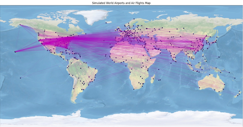
Unfortunately, we can’t share the details about the AWS backbone network including the data we used to train the model. To still provide you with some code that makes it straightforward to get started solving your network prediction problems, we share a synthetic traffic prediction problem instead. We have created a Jupyter notebook that generates synthetic airport traffic data. This dataset simulates a global air transportation network using major world airports, creating fictional airlines and flights with predefined capacities. The following figure illustrates these major airports and the simulated flight routes derived from our synthetic data.

Our synthetic data includes: major world airports, simulated airlines and flights with predefined capacities for cargo demands, and generated air cargo demands between airport pairs, which will be delivered by simulated flights.
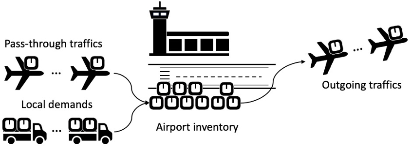
We employ a simple routing policy to distribute these demands evenly across all shortest paths between two airports. This policy is intentionally hidden from our model, mimicking the real-world scenarios where the exact routing mechanisms are not always known. If flight capacity is insufficient to meet incoming demands, we simulate the excess as inventory stored at the airport. The total inventory at each airport serves as our prediction target. Unlike real air transportation networks, we didn’t follow a hub-and-spoke topology. Instead, our synthetic network uses a point-to-point structure. Using this synthetic air transportation dataset, we now demonstrate a node time series regression task, predicting the total inventory at each airport every day. As illustrated in the following figure, the total inventory amount at an airport is influenced by its own local demands, the traffic passing through it, and the capacity that it can output. By design, the output capacity of an airport is limited to make sure that most airport-to-airport demands require multiple-hop fulfillment.

In the remainder of this section, we cover the data preprocessing steps necessary for using the GraphStorm framework, before customizing a GNN model for our application. Towards the end of the post, we also provide an architecture for an operational safety system built using GraphStorm and in an environment of AWS services.
Data preprocessing for graph time series forecasting
To use GraphStorm for node time series regression, we need to structure our synthetic air traffic dataset according to GraphStorm’s input data format requirements. This involves preparing three key components: a set of node tables, a set of edge tables, and a JSON file describing the dataset.
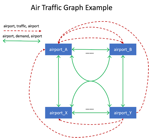
We abstract the synthetic air traffic network into a graph with one node type (airport) and two edge types. The first edge type, airport, demand, airport, represents demand between any pair of airports. The second one, airport, traffic, airport, captures the amount of traffic sent between connected airports.
The following diagram illustrates this graph structure.

Our airport nodes have two types of associated features: static features (longitude and latitude) and time series features (daily total inventory amount). For each edge, the src_code and dst_code capture the source and destination airport codes. The edge features also include a demand and a traffic time series. Finally, edges for connected airports also hold the capacity as a static feature.
The synthetic data generation notebook also creates a JSON file, which describes the air traffic data and provides instructions for GraphStorm’s graph construction tool to follow. Using these artifacts, we can employ the graph construction tool to convert the air traffic graph data into a distributed DGL graph. In this format:
- Demand and traffic time series data is stored as E*T tensors in edges, where E is the number of edges of a given type, and T is the number of days in our dataset.
- Inventory amount time series data is stored as an N*T tensor in nodes, where N is the number of airport nodes.
This preprocessing step makes sure our data is optimally structured for time series forecasting using GraphStorm.
Model
To predict the next total inventory amount for each airport, we employ GNN models, which are well-suited for capturing these complex relationships. Specifically, we use GraphStorm’s Relational Graph Convolutional Network (RGCN) module as our GNN model. This allows us to effectively pass information (demands and traffic) among airports in our network. To support the sliding-window prediction method we described earlier, we created a customized RGCN model.
The detailed implementation of the node time series regression model can be found in the Python file. In the following sections, we explain a few key implementation points.
Customized RGCN model
The GraphStorm v0.4 release adds support for edge features. This means that we can use a for-loop to iterate along the T dimensions in the time series tensor, thereby implementing the sliding-window method in the forward() function during model training, as shown in the following pseudocode:
The actual code of the forward() function is in the following code snippet.
In contrast, because the inference step needs to use the autoregressive sliding-window method, we implement a one-step prediction function in the predict() routine:
The actual code of the predict() function is in the following code snippet.
Customized node trainer
GraphStorm’s default node trainer (GSgnnNodePredctionTrainer), which handles the model training loop, can’t process the time series feature requirement. Therefore, we implement a customized node trainer by inheriting the GSgnnNodePredctionTrainer and use our own customized node_mini_batch_gnn_predict() method. This is shown in the following code snippet.
Customized node_mini_batch_predict() method
The customized node_mini_batch_predict() method calls the customized model’s predict() method, passing the two additional arguments that are specific to our use case. These are used to determine whether the autoregressive property is used or not, along with the current prediction step for appropriate indexing (see the following code snippet).
Customized node predictor (inferrer)
Similar to the node trainer, GraphStorm’s default node inference class, which drives the inference pipeline (GSgnnNodePredictionInferrer), can’t handle the time series feature processing we need in this application. We therefore create a customized node inferrer by inheriting GSgnnNodePredictionInferrer, and add two specific arguments. In this customized inferrer, we use a for-loop to iterate over the T dimensions of the time series feature tensor. Unlike the for-loop we used in model training, the inference loop uses the predicted values in subsequent prediction steps (this is shown in the following code snippet).
So far, we have focused on the node prediction example with our dataset and modeling. However, our approach allows for various other prediction tasks, such as:
- Forecasting traffic between specific airport pairs.
- More complex scenarios like predicting potential airport congestion or increased utilization of alternative routes when reducing or eliminating flights between certain airports.
With the customized model and pipeline classes, we can use the following Jupyter notebook to run the overall training and inference pipeline for our airport inventory amount prediction task. We encourage you to explore these possibilities, adapt the provided example to your specific use cases or research interests, and refer to our Jupyter notebooks for a comprehensive understanding of how to use GraphStorm APIs for various GML tasks.
System architecture for GNN-based network traffic prediction
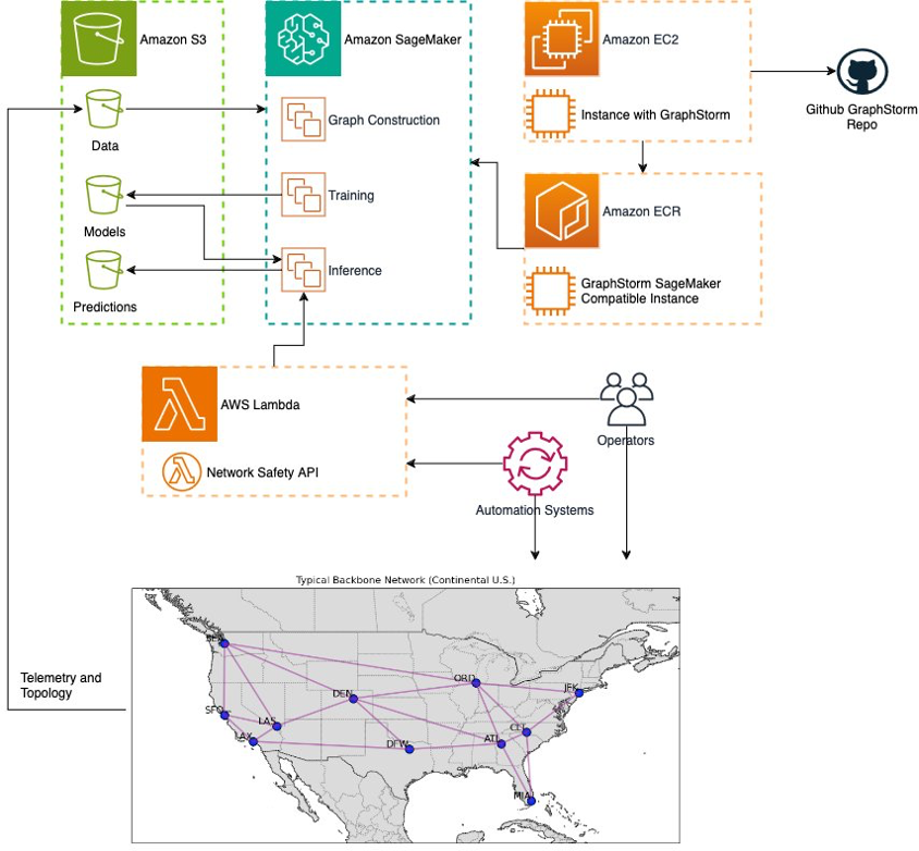
In this section, we propose a system architecture for enhancing operational safety within a complex network, such as the ones we discussed earlier. Specifically, we employ GraphStorm within an AWS environment to build, train, and deploy graph models. The following diagram shows the various components we need to achieve the safety functionality.

The complex system in question is represented by the network shown at the bottom of the diagram, overlaid on the map of the continental US. This network emits telemetry data that can be stored on Amazon Simple Storage Service (Amazon S3) in a dedicated bucket. The evolving topology of the network should also be extracted and stored.
On the top right of the preceding diagram, we show how Amazon Elastic Compute Cloud (Amazon EC2) instances can be configured with the necessary GraphStorm dependencies using direct access to the project’s GitHub repository. After they’re configured, we can build GraphStorm Docker images on them. These images then can be put on Amazon Elastic Container Registry (Amazon ECR) and be made available to other services (for example, Amazon SageMaker).
During training, SageMaker jobs use those instances along with the network data to train a traffic prediction model such as the one we demonstrated in this post. The trained model can then be stored on Amazon S3. It might be necessary to repeat this training process periodically, to make sure that the model’s performance keeps up with changes to the network dynamics (such as modifications to the routing schemes).
Above the network representation, we show two possible actors: operators and automation systems. These actors call on a network safety API implemented in AWS Lambda to make sure that the actions they intend to take are safe for the anticipated time horizon (for example, 1 hour, 6 hours, 24 hours). To provide an answer, the Lambda function uses the on-demand inference capabilities of SageMaker. During inference, SageMaker uses the pre-trained model to produce the necessary traffic predictions. These predictions can also be stored on Amazon S3 to continuously monitor the model’s performance over time, triggering training jobs when significant drift is detected.
Conclusion
Maintaining operational safety for the AWS backbone network, while supporting the dynamic needs of our global customer base, is a unique challenge. In this post, we demonstrated how the GML framework GraphStorm can be effectively applied to predict traffic patterns and potential congestion risks in such complex networks. By framing our network as a heterogeneous graph and using GNNs, we’ve shown that it’s possible to capture the intricate interdependencies and dynamic nature of network traffic. Our approach, tested on both synthetic data and the actual AWS backbone network, has demonstrated significant improvements over traditional time series forecasting methods, with a 35% reduction in prediction error compared to classical approaches like XGBoost.
The proposed system architecture, integrating GraphStorm with various AWS services like Amazon S3, Amazon EC2, SageMaker, and Lambda, provides a scalable and efficient framework for implementing this approach in production environments. This setup allows for continuous model training, rapid inference, and seamless integration with existing operational workflows.
We will keep you posted about our progress in taking our solution to production, and share the benefit for AWS customers.
We encourage you to explore the provided Jupyter notebooks, adapt our approach to your specific use cases, and contribute to the ongoing development of graph-based ML techniques for managing complex networked systems. To learn how to use GraphStorm to solve a broader class of ML problems on graphs, see the GitHub repo.
About the Authors
 Jian Zhang is a Senior Applied Scientist who has been using machine learning techniques to help customers solve various problems, such as fraud detection, decoration image generation, and more. He has successfully developed graph-based machine learning, particularly graph neural network, solutions for customers in China, the US, and Singapore. As an enlightener of AWS graph capabilities, Zhang has given many public presentations about GraphStorm, the GNN, the Deep Graph Library (DGL), Amazon Neptune, and other AWS services.
 Fabien Chraim is a Principal Research Scientist in AWS networking. Since 2017, he’s been researching all aspects of network automation, from telemetry and anomaly detection to root causing and actuation. Before Amazon, he co-founded and led research and development at Civil Maps (acquired by Luminar). He holds a PhD in electrical engineering and computer sciences from UC Berkeley.
 Patrick Taylor is a Senior Data Scientist in AWS networking. Since 2020, he has focused on impact reduction and risk management in networking software systems and operations research in networking operations teams. Previously, Patrick was a data scientist specializing in natural language processing and AI-driven insights at Hyper Anna (acquired by Alteryx) and holds a Bachelor’s degree from the University of Sydney.
 Xiang Song is a Senior Applied Scientist at AWS AI Research and Education (AIRE), where he develops deep learning frameworks including GraphStorm, DGL, and DGL-KE. He led the development of Amazon Neptune ML, a new capability of Neptune that uses graph neural networks for graphs stored in graph database. He is now leading the development of GraphStorm, an open source graph machine learning framework for enterprise use cases. He received his PhD in computer systems and architecture at the Fudan University, Shanghai, in 2014.
 Florian Saupe is a Principal Technical Product Manager at AWS AI/ML research supporting science teams like the graph machine learning group, and ML Systems teams working on large scale distributed training, inference, and fault resilience. Before joining AWS, Florian lead technical product management for automated driving at Bosch, was a strategy consultant at McKinsey & Company, and worked as a control systems and robotics scientist—a field in which he holds a PhD.