Time series forecasting with Amazon SageMaker AutoML

Time series forecasting is a critical component in various industries for making informed decisions by predicting future values of time-dependent data. A time series is a sequence of data points recorded at regular time intervals, such as daily sales revenue, hourly temperature readings, or weekly stock market prices. These forecasts are pivotal for anticipating trends and future demands in areas such as product demand, financial markets, energy consumption, and many more.

However, creating accurate and reliable forecasts poses significant challenges because of factors such as seasonality, underlying trends, and external influences that can dramatically impact the data. Additionally, traditional forecasting models often require extensive domain knowledge and manual tuning, which can be time-consuming and complex.

In this blog post, we explore a comprehensive approach to time series forecasting using the Amazon SageMaker AutoMLV2 Software Development Kit (SDK). SageMaker AutoMLV2 is part of the SageMaker Autopilot suite, which automates the end-to-end machine learning workflow from data preparation to model deployment. Throughout this blog post, we will be talking about AutoML to indicate SageMaker Autopilot APIs, as well as Amazon SageMaker Canvas AutoML capabilities. We’ll walk through the data preparation process, explain the configuration of the time series forecasting model, detail the inference process, and highlight key aspects of the project. This methodology offers insights into effective strategies for forecasting future data points in a time series, using the power of machine learning without requiring deep expertise in model development. The code for this post can be found in the GitHub repo.

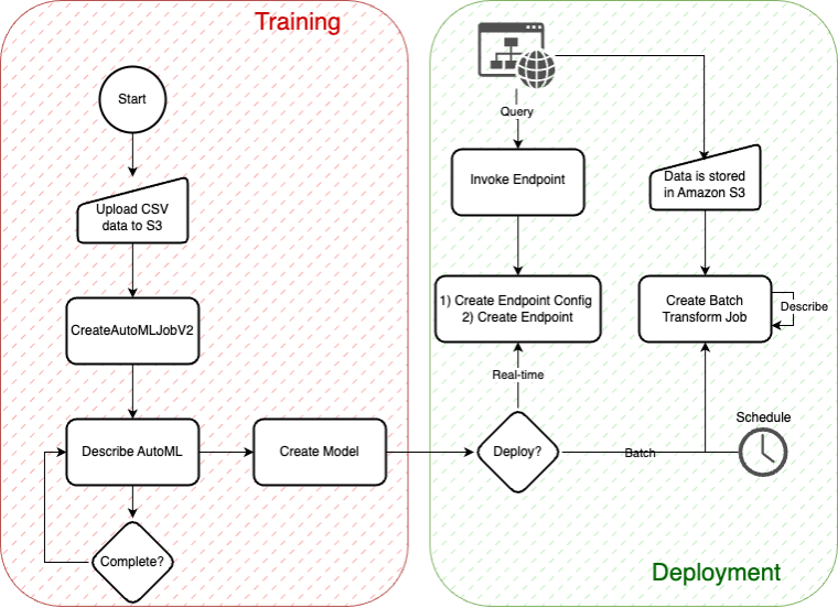
The following diagram depicts the basic AutoMLV2 APIs, all of which are relevant to this post. The diagram shows the workflow for building and deploying models using the AutoMLV2 API. In the training phase, CSV data is uploaded to Amazon S3, followed by the creation of an AutoML job, model creation, and checking for job completion. The deployment phase allows you to choose between real-time inference via an endpoint or batch inference using a scheduled transform job that stores results in S3.

1. Data preparation

The foundation of any machine learning project is data preparation. For this project, we used a synthetic dataset containing time series data of product sales across various locations, focusing on attributes such as product code, location code, timestamp, unit sales, and promotional information. The dataset can be found in an Amazon-owned, public Amazon Simple Storage Service (Amazon S3) dataset.

When preparing your CSV file for input into a SageMaker AutoML time series forecasting model, you must ensure that it includes at least three essential columns (as described in the SageMaker AutoML V2 documentation):

1. Item identifier attribute name: This column contains unique identifiers for each item or entity for which predictions are desired. Each identifier distinguishes the individual data series within the dataset. For example, if you’re forecasting sales for multiple products, each product would have a unique identifier.
2. Target attribute name: This column represents the numerical values that you want to forecast. These could be sales figures, stock prices, energy usage amounts, and so on. It’s crucial that the data in this column is numeric because the forecasting models predict quantitative outcomes.
3. Timestamp attribute name: This column indicates the specific times when the observations were recorded. The timestamp is essential for analyzing the data in a chronological context, which is fundamental to time series forecasting. The timestamps should be in a consistent and appropriate format that reflects the regularity of your data (for example, daily or hourly).

All other columns in the dataset are optional and can be used to include additional time-series related information or metadata about each item. Therefore, your CSV file should have columns named according to the preceding attributes (item identifier, target, and timestamp) as well as any other columns needed to support your use case For instance, if your dataset is about forecasting product demand, your CSV might look something like this:

• Product_ID (item identifier): Unique product identifiers.
• Sales (target): Historical sales data to be forecasted.
• Date (timestamp): The dates on which sales data was recorded.

The process of splitting the training and test data in this project uses a methodical and time-aware approach to ensure that the integrity of the time series data is maintained. Here’s a detailed overview of the process:

Ensuring timestamp integrity

The first step involves converting the timestamp column of the input dataset to a datetime format using pd.to_datetime. This conversion is crucial for sorting the data chronologically in subsequent steps and for ensuring that operations on the timestamp column are consistent and accurate.

Sorting the data

The sorted dataset is critical for time series forecasting, because it ensures that data is processed in the correct temporal order. The input_data DataFrame is sorted based on three columns: product_code, location_code, and timestamp. This multi-level sort guarantees that the data is organized first by product and location, and then chronologically within each product-location grouping. This organization is essential for the logical partitioning of data into training and test sets based on time.

Splitting into training and test sets

The splitting mechanism is designed to handle each combination of product_code and location_code separately, respecting the unique temporal patterns of each product-location pair. For each group:

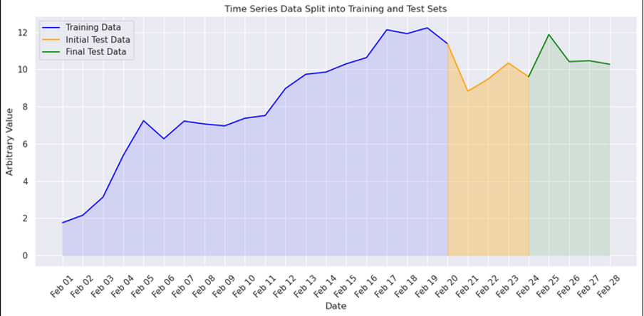
• The initial test set is determined by selecting the last eight timestamps (yellow + green below). This subset represents the most recent data points that are candidates for testing the model’s forecasting ability.
• The final test set is refined by removing the last four timestamps from the initial test set, resulting in a test dataset that includes the four timestamps immediately preceding the latest data (green below). This strategy ensures the test set is representative of the near-future periods the model is expected to predict, while also leaving out the most recent data to simulate a realistic forecasting scenario.
• The training set comprises the remaining data points, excluding the last eight timestamps (blue below). This ensures the model is trained on historical data that precedes the test period, avoiding any data leakage and ensuring that the model learns from genuinely past observations.

This process is visualized in the following figure with an arbitrary value on the Y axis and the days of February on the X axis.

The test dataset is used to evaluate the performance of the trained model and compute various loss metrics, such as mean absolute error (MAE) and root-mean-squared error (RMSE). These metrics quantify the model’s accuracy in forecasting the actual values in the test set, providing a clear indication of the model’s quality and its ability to make accurate predictions. The evaluation process is detailed in the “Inference: Batch, real-time, and asynchronous” section, where we discuss the comprehensive approach to model evaluation and conditional model registration based on the computed metrics.

Creating and saving the datasets

After the data for each product-location group is categorized into training and test sets, the subsets are aggregated into comprehensive training and test DataFrames using pd.concat. This aggregation step combines the individual DataFrames stored in train_dfs and test_dfs lists into two unified DataFrames:

• train_df for training data
• test_df for testing data

Finally, the DataFrames are saved to CSV files (train.csv for training data and test.csv for test data), making them accessible for model training and evaluation processes. This saving step not only facilitates a clear separation of data for modelling purposes but also enables reproducibility and sharing of the prepared datasets.

Summary

This data preparation strategy meticulously respects the chronological nature of time series data and ensures that the training and test sets are appropriately aligned with real-world forecasting scenarios. By splitting the data based on the last known timestamps and carefully excluding the most recent periods from the training set, the approach mimics the challenge of predicting future values based on past observations, thereby setting the stage for a robust evaluation of the forecasting model’s performance.

2. Training a model with AutoMLV2

SageMaker AutoMLV2 reduces the resources needed to train, tune, and deploy machine learning models by automating the heavy lifting involved in model development. It provides a straightforward way to create high-quality models tailored to your specific problem type, be it classification, regression, or forecasting, among others. In this section, we delve into the steps to train a time series forecasting model with AutoMLV2.

Step 1: Define the tine series forecasting configuration

The first step involves defining the problem configuration. This configuration guides AutoMLV2 in understanding the nature of your problem and the type of solution it should seek, whether it involves classification, regression, time-series classification, computer vision, natural language processing, or fine-tuning of large language models. This versatility is crucial because it allows AutoMLV2 to adapt its approach based on the specific requirements and complexities of the task at hand. For time series forecasting, the configuration includes details such as the frequency of forecasts, the horizon over which predictions are needed, and any specific quantiles or probabilistic forecasts. Configuring the AutoMLV2 job for time series forecasting involves specifying parameters that would best use the historical sales data to predict future sales.

The AutoMLTimeSeriesForecastingConfig is a configuration object in the SageMaker AutoMLV2 SDK designed specifically for setting up time series forecasting tasks. Each argument provided to this configuration object tailors the AutoML job to the specifics of your time series data and the forecasting objectives.

time_series_config = AutoMLTimeSeriesForecastingConfig(
    forecast_frequency='W',
    forecast_horizon=4,
    item_identifier_attribute_name='product_code',
    target_attribute_name='unit_sales',
    timestamp_attribute_name='timestamp',
    ...
)

The following is a detailed explanation of each configuration argument used in your time series configuration:

• forecast_frequency
  • Description: Specifies how often predictions should be made.
  • Value ‘W’: Indicates that forecasts are expected on a weekly basis. The model will be trained to understand and predict data as a sequence of weekly observations. Valid intervals are an integer followed by Y (year), M (month), W (week), D (day), H (hour), and min (minute). For example, 1D indicates every day and 15min indicates every 15 minutes. The value of a frequency must not overlap with the next larger frequency. For example, you must use a frequency of 1H instead of 60min.

• forecast_horizon
  • Description: Defines the number of future time-steps the model should predict.
  • Value 4: The model will forecast four time-steps into the future. Given the weekly frequency, this means the model will predict the next four weeks of data from the last known data point.

• forecast_quantiles
  • Description: Specifies the quantiles at which to generate probabilistic forecasts.
  • Values [p50,p60,p70,p80,p90]: These quantiles represent the 50th, 60th, 70th, 80th, and 90th percentiles of the forecast distribution, providing a range of possible outcomes and capturing forecast uncertainty. For instance, the p50 quantile (median) might be used as a central forecast, while the p90 quantile provides a higher-end forecast, where 90% of the actual data is expected to fall below the forecast, accounting for potential variability.

• filling
  • Description: Defines how missing data should be handled before training; specifying filling strategies for different scenarios and columns.
  • Value filling_config: This should be a dictionary detailing how to fill missing values in your dataset, such as filling missing promotional data with zeros or specific columns with predefined values. This ensures the model has a complete dataset to learn from, improving its ability to make accurate forecasts.

• item_identifier_attribute_name
  • Description: Specifies the column that uniquely identifies each time series in the dataset.
  • Value ’product_code’: This setting indicates that each unique product code represents a distinct time series. The model will treat data for each product code as a separate forecasting problem.

• target_attribute_name
  • Description: The name of the column in your dataset that contains the values you want to predict.
  • Value unit_sales: Designates the unit_sales column as the target variable for forecasts, meaning the model will be trained to predict future sales figures.

• timestamp_attribute_name
  • Description: The name of the column indicating the time point for each observation.
  • Value ‘timestamp’: Specifies that the timestamp column contains the temporal information necessary for modeling the time series.

• grouping_attribute_names
  • Description: A list of column names that, in combination with the item identifier, can be used to create composite keys for forecasting.
  • Value [‘location_code’]: This setting means that forecasts will be generated for each combination of product_code and location_code. It allows the model to account for location-specific trends and patterns in sales data.

The configuration provided instructs the SageMaker AutoML to train a model capable of weekly sales forecasts for each product and location, accounting for uncertainty with quantile forecasts, handling missing data, and recognizing each product-location pair as a unique series. This detailed setup aims to optimize the forecasting model’s relevance and accuracy for your specific business context and data characteristics.

Step 2: Initialize the AutoMLV2 job

Next, initialize the AutoMLV2 job by specifying the problem configuration, the AWS role with permissions, the SageMaker session, a base job name for identification, and the output path where the model artifacts will be stored.

automl_sm_job = AutoMLV2(
    problem_config=time_series_config,
    role=role,
    sagemaker_session=sagemaker_session,
    base_job_name='time-series-forecasting-job',
    output_path=f's3://{bucket}/{prefix}/output'
)

Step 3: Fit the model

To start the training process, call the fit method on your AutoMLV2 job object. This method requires specifying the input data’s location in Amazon S3 and whether SageMaker should wait for the job to complete before proceeding further. During this step, AutoMLV2 will automatically pre-process your data, select algorithms, train multiple models, and tune them to find the best solution.

automl_sm_job.fit(
    inputs=[AutoMLDataChannel(s3_data_type='S3Prefix', s3_uri=train_uri, channel_type='training')],
    wait=True,
    logs=True
)

Please note that model fitting may take several hours, depending on the size of your dataset and compute budget. A larger compute budget allows for more powerful instance types, which can accelerate the training process. In this situation, provided you’re not running this code as part of the provided SageMaker notebook (which handles the order of code cell processing correctly), you will need to implement some custom code that monitors the training status before retrieving and deploying the best model.

3. Deploying a model with AutoMLV2

Deploying a machine learning model into production is a critical step in your machine learning workflow, enabling your applications to make predictions from new data. SageMaker AutoMLV2 not only helps build and tune your models but also provides a seamless deployment experience. In this section, we’ll guide you through deploying your best model from an AutoMLV2 job as a fully managed endpoint in SageMaker.

Step 1: Identify the best model and extract name

After your AutoMLV2 job completes, the first step in the deployment process is to identify the best performing model, also known as the best candidate. This can be achieved by using the best_candidate method of your AutoML job object. You can either use this method immediately after fitting the AutoML job or specify the job name explicitly if you’re operating on a previously completed AutoML job.

# Option 1: Directly after fitting the AutoML job
best_candidate = automl_sm_job.best_candidate()

# Option 2: Specifying the job name directly
best_candidate = automl_sm_job.best_candidate(job_name='your-auto-ml-job-name')

best_candidate_name = best_candidate['CandidateName']

Step 2: Create a SageMaker model

Before deploying, create a SageMaker model from the best candidate. This model acts as a container for the artifacts and metadata necessary to serve predictions. Use the create_model method of the AutoML job object to complete this step.

endpoint_name = f"ep-{best_candidate_name}-automl-ts"

# Create a SageMaker model from the best candidate
automl_sm_model = automl_sm_job.create_model(name=best_candidate_name, candidate=best_candidate)

4. Inference: Batch, real-time, and asynchronous

For deploying the trained model, we explore batch, real-time, and asynchronous inference methods to cater to different use cases.

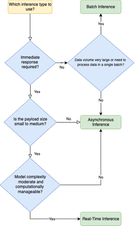
The following figure is a decision tree to help you decide what type of endpoint to use. The diagram outlines a decision-making process for selecting between batch, asynchronous, or real-time inference endpoints. Starting with the need for immediate responses, it guides you through considerations like the size of the payload and the computational complexity of the model. Depending on these factors, you can choose a faster option with lower computational requirements or a slower batch process for larger datasets.

Batch inference using SageMaker pipelines

• Usage: Ideal for generating forecasts in bulk, such as monthly sales predictions across all products and locations.
• Process: We used SageMaker’s batch transform feature to process a large dataset of historical sales data, outputting forecasts for the specified horizon.

The inference pipeline used for batch inference demonstrates a comprehensive approach to deploying, evaluating, and conditionally registering a machine learning model for time series forecasting using SageMaker. This pipeline is structured to ensure a seamless flow from data preprocessing, through model inference, to post-inference evaluation and conditional model registration. Here’s a detailed breakdown of its construction:

• Batch tranform step
  • Transformer Initialization: A Transformer object is created, specifying the model to use for batch inference, the compute resources to allocate, and the output path for the results.
  • Transform step creation: This step invokes the transformer to perform batch inference on the specified input data. The step is configured to handle data in CSV format, a common choice for structured time series data.

• Evaluation step
  • Processor setup: Initializes an SKLearn processor with the specified role, framework version, instance count, and type. This processor is used for the evaluation of the model’s performance.
  • Evaluation processing: Configures the processing step to use the SKLearn processor, taking the batch transform output and test data as inputs. The processing script (evaluation.py) is specified here, which will compute evaluation metrics based on the model’s predictions and the true labels.
  • Evaluation strategy: We adopted a comprehensive evaluation approach, using metrics like mean absolute error (MAE) and root-means squared error (RMSE) to quantify the model’s accuracy and adjusting the forecasting configuration based on these insights.
  • Outputs and property files: The evaluation step produces an output file (evaluation_metrics.json) that contains the computed metrics. This file is stored in Amazon S3 and registered as a property file for later access in the pipeline.

• Conditional model registration
  • Model metrics setup: Defines the model metrics to be associated with the model package, including statistics and explainability reports sourced from specified Amazon S3 URIs.
  • Model registration: Prepares for model registration by specifying content types, inference and transform instance types, model package group name, approval status, and model metrics.
  • Conditional registration step: Implements a condition based on the evaluation metrics (for example, MAE). If the condition (for example, MAE is greater than or equal to threshold) is met, the model is registered; otherwise, the pipeline concludes without model registration.

• Pipeline creation and runtime
  • Pipeline definition: Assembles the pipeline by naming it and specifying the sequence of steps to run: batch transform, evaluation, and conditional registration.
  • Pipeline upserting and runtime: The pipeline.upsert method is called to create or update the pipeline based on the provided definition, and pipeline.start() runs the pipeline.

The following figure is an example of the SageMaker Pipeline directed acyclic graph (DAG).

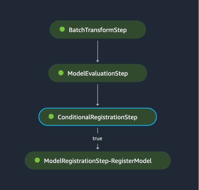
This pipeline effectively integrates several stages of the machine learning lifecycle into a cohesive workflow, showcasing how Amazon SageMaker can be used to automate the process of model deployment, evaluation, and conditional registration based on performance metrics. By encapsulating these steps within a single pipeline, the approach enhances efficiency, ensures consistency in model evaluation, and streamlines the model registration process—all while maintaining the flexibility to adapt to different models and evaluation criteria.

Inferencing with Amazon SageMaker Endpoint in (near) real-time

But what if you want to run inference in real-time or asynchronously? SageMaker real-time endpoint inference offers the capability to deliver immediate predictions from deployed machine learning models, crucial for scenarios demanding quick decision making. When an application sends a request to a SageMaker real-time endpoint, it processes the data in real time and returns the prediction almost immediately. This setup is optimal for use cases that require near-instant responses, such as personalized content delivery, immediate fraud detection, and live anomaly detection.

• Usage: Suited for on-demand forecasts, such as predicting next week’s sales for a specific product at a particular location.
• Process: We deployed the model as a SageMaker endpoint, allowing us to make real-time predictions by sending requests with the required input data.

Deployment involves specifying the number of instances and the instance type to serve predictions. This step creates an HTTPS endpoint that your applications can invoke to perform real-time predictions.

# Deploy the model to a SageMaker endpoint
predictor = automl_sm_model.deploy(initial_instance_count=1, endpoint_name=endpoint_name, instance_type='ml.m5.xlarge')

The deployment process is asynchronous, and SageMaker takes care of provisioning the necessary infrastructure, deploying your model, and ensuring the endpoint’s availability and scalability. After the model is deployed, your applications can start sending prediction requests to the endpoint URL provided by SageMaker.

While real-time inference is suitable for many use cases, there are scenarios where a slightly relaxed latency requirement can be beneficial. SageMaker Asynchronous Inference provides a queue-based system that efficiently handles inference requests, scaling resources as needed to maintain performance. This approach is particularly useful for applications that require processing of larger datasets or complex models, where the immediate response is not as critical.

• Usage: Examples include generating detailed reports from large datasets, performing complex calculations that require significant computational time, or processing high-resolution images or lengthy audio files. This flexibility makes it a complementary option to real-time inference, especially for businesses that face fluctuating demand and seek to maintain a balance between performance and cost.
• Process: The process of using asynchronous inference is straightforward yet powerful. Users submit their inference requests to a queue, from which SageMaker processes them sequentially. This queue-based system allows SageMaker to efficiently manage and scale resources according to the current workload, ensuring that each inference request is handled as promptly as possible.

Clean up

To avoid incurring unnecessary charges and to tidy up resources after completing the experiments or running the demos described in this post, follow these steps to delete all deployed resources:

1. Delete the SageMaker endpoints: To delete any deployed real-time or asynchronous endpoints, use the SageMaker console or the AWS SDK. This step is crucial as endpoints can accrue significant charges if left running.
2. Delete the SageMaker Pipeline: If you have set up a SageMaker Pipeline, delete it to ensure that there are no residual executions that might incur costs.
3. Delete S3 artifacts: Remove all artifacts stored in your S3 buckets that were used for training, storing model artifacts, or logging. Ensure you delete only the resources related to this project to avoid data loss.
4. Clean up any additional resources: Depending on your specific implementation and additional setup modifications, there may be other resources to consider, such as roles or logs. Check your AWS Management Console for any resources that were created and delete them if they are no longer needed.

Conclusion

This post illustrates the effectiveness of Amazon SageMaker AutoMLV2 for time series forecasting. By carefully preparing the data, thoughtfully configuring the model, and using both batch and real-time inference, we demonstrated a robust methodology for predicting future sales. This approach not only saves time and resources but also empowers businesses to make data-driven decisions with confidence.

If you’re inspired by the possibilities of time series forecasting and want to experiment further, consider exploring the SageMaker Canvas UI. SageMaker Canvas provides a user-friendly interface that simplifies the process of building and deploying machine learning models, even if you don’t have extensive coding experience.

Visit the SageMaker Canvas page to learn more about its capabilities and how it can help you streamline your forecasting projects. Begin your journey towards more intuitive and accessible machine learning solutions today!

About the Authors

Nick McCarthy is a Senior Machine Learning Engineer at AWS, based in London. He has worked with AWS clients across various industries including healthcare, finance, sports, telecoms and energy to accelerate their business outcomes through the use of AI/ML. Outside of work he loves to spend time travelling, trying new cuisines and reading about science and technology. Nick has a Bachelors degree in Astrophysics and a Masters degree in Machine Learning.

Davide Gallitelli is a Senior Specialist Solutions Architect for AI/ML in the EMEA region. He is based in Brussels and works closely with customers throughout Benelux. He has been a developer since he was very young, starting to code at the age of 7. He started learning AI/ML at university, and has fallen in love with it since then.