使用 Amazon SageMaker 构建语义内容推荐系统


训练和部署内容推荐模型
在本模块中,您将使用内置的 Amazon SageMaker k-Nearest Neighbors (k-NN) 算法来训练内容推荐模型。
Amazon SageMaker k-Nearest Neighbors (k-NN) 是一种基于索引的非参数监督学习算法,可用于分类和回归任务。对于分类,该算法查询距离目标最近的 k 个点,并返回它们的类别中最频繁的标签作为预测标签。对于回归问题,该算法返回 k 个最近邻返回的预测值的平均值。
使用 k-NN 算法进行训练分为三个步骤:采样、降维和索引构建。采样可以减小初始数据集的大小,使其适合内存。对于降维,该算法降低数据的特征维度,以减少 k-NN 模型在内存中的占用和推理延迟。我们提供了两种降维方法:随机投影和快速 Johnson-Lindenstrauss 变换。通常,您对高维 (d > 1000) 数据集应用降维,以避免“维度诅咒”,即随着维度增加,数据变得稀疏,从而给统计分析带来困难。k-NN 训练的主要目标是构建索引。索引可以高效查找值或类别标签尚未确定的点与用于推理的 k 个最近点之间的距离。
在接下来的步骤中,您将为训练作业指定 k-NN 算法,设置超参数值来优化模型,然后运行模型。然后,将模型部署到由 Amazon SageMaker 管理的端点,以进行预测。
时长
20 分钟
步骤 1:创建并运行训练作业
在之前的模块中,您创建了主题向量。在本模块中,您将构建并部署内容推荐模块,该模块保留主题向量的索引。
首先,创建一个字典,将随机排列的标签映射到训练数据中的原始标签。在 Notebook 中,复制粘贴以下代码,然后点击 Run(运行)。
labels = newidx
labeldict = dict(zip(newidx,idx))接下来,使用以下代码将训练数据存储到您的 S3 存储桶中:
import io
import sagemaker.amazon.common as smac


print('train_features shape = ', predictions.shape)
print('train_labels shape = ', labels.shape)
buf = io.BytesIO()
smac.write_numpy_to_dense_tensor(buf, predictions, labels)
buf.seek(0)

bucket = BUCKET
prefix = PREFIX
key = 'knn/train'
fname = os.path.join(prefix, key)
print(fname)
boto3.resource('s3').Bucket(bucket).Object(fname).upload_fileobj(buf)
s3_train_data = 's3://{}/{}/{}'.format(bucket, prefix, key)
print('uploaded training data location: {}'.format(s3_train_data))然后,使用以下辅助函数创建一个 k-NN 估计器,类似于您在模块 3 中创建的 NTM 估计器。
def trained_estimator_from_hyperparams(s3_train_data, hyperparams, output_path, s3_test_data=None):
    """
    Create an Estimator from the given hyperparams, fit to training data,
    and return a deployed predictor

    """
    # set up the estimator
    knn = sagemaker.estimator.Estimator(get_image_uri(boto3.Session().region_name, "knn"),
        get_execution_role(),
        train_instance_count=1,
        train_instance_type='ml.c4.xlarge',
        output_path=output_path,
        sagemaker_session=sagemaker.Session())
    knn.set_hyperparameters(**hyperparams)

    # train a model. fit_input contains the locations of the train and test data
    fit_input = {'train': s3_train_data}
    knn.fit(fit_input)
    return knn

hyperparams = {
    'feature_dim': predictions.shape[1],
    'k': NUM_NEIGHBORS,
    'sample_size': predictions.shape[0],
    'predictor_type': 'classifier' ,
    'index_metric':'COSINE'
}
output_path = 's3://' + bucket + '/' + prefix + '/knn/output'
knn_estimator = trained_estimator_from_hyperparams(s3_train_data, hyperparams, output_path)在训练作业运行时,仔细查看辅助函数中的参数。
Amazon SageMaker k-NN 算法提供了多种不同的距离度量方法来计算最近邻。自然语言处理中常用的一种度量是余弦距离。在数学上,两个向量 A 和 B 之间的余弦“相似度”由以下公式给出:
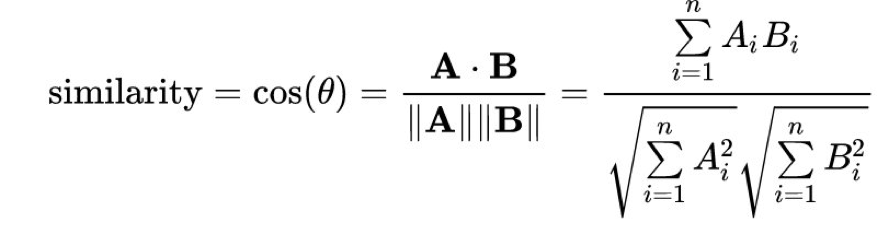
通过将 index_metric 设置为 COSINE,Amazon SageMaker 将自动使用余弦相似度来计算最近邻。默认距离为 L2 范数,即标准欧几里得距离。请注意,截至本文撰写时,COSINE 仅支持 faiss.IVFFlat 索引类型,而不支持 faiss.IVFPQ 索引方法。
您应该会在终端中看到以下输出。
Completed - Training job completed大功告成!由于您希望该模型在给定特定测试主题时返回最近邻,因此需要将其部署为实时托管端点。
步骤 2:部署内容推荐模型
与 NTM 模型一样,为 k-NN 模型定义以下辅助函数来启动端点。在辅助函数中,接受令牌 applications/jsonlines; verbose=true 会让 k-NN 模型返回所有余弦距离,而不仅仅是最近邻。要构建推荐引擎,您需要从模型中获取 top-k 建议,为此您需要将 verbose 参数设置为 true,而不是默认的 false。
将以下代码复制并粘贴到 Notebook 中,然后点击 Run(运行)。
def predictor_from_estimator(knn_estimator, estimator_name, instance_type, endpoint_name=None):
    knn_predictor = knn_estimator.deploy(initial_instance_count=1, instance_type=instance_type,
                                        endpoint_name=endpoint_name,
                                        accept="application/jsonlines; verbose=true")
    knn_predictor.content_type = 'text/csv'
    knn_predictor.serializer = csv_serializer
    knn_predictor.deserializer = json_deserializer
    return knn_predictor
import time

instance_type = 'ml.m4.xlarge'
model_name = 'knn_%s'% instance_type
endpoint_name = 'knn-ml-m4-xlarge-%s'% (str(time.time()).replace('.','-'))
print('setting up the endpoint..')
knn_predictor = predictor_from_estimator(knn_estimator, model_name, instance_type, endpoint_name=endpoint_name)接下来,对测试数据进行预处理,以便运行推理。
将以下代码复制并粘贴到 Notebook 中,然后点击 Run(运行)。
def preprocess_input(text):
    text = strip_newsgroup_header(text)
    text = strip_newsgroup_quoting(text)
    text = strip_newsgroup_footer(text)
    return text

test_data_prep = []
for i in range(len(newsgroups_test)):
    test_data_prep.append(preprocess_input(newsgroups_test[i]))
test_vectors = vectorizer.fit_transform(test_data_prep)

test_vectors = np.array(test_vectors.todense())
test_topics = []
for vec in test_vectors:
    test_result = ntm_predictor.predict(vec)
    test_topics.append(test_result['predictions'][0]['topic_weights'])

topic_predictions = []
for topic in test_topics:
    result = knn_predictor.predict(topic)
    cur_predictions = np.array([int(result['labels'][i]) for i in range(len(result['labels']))])
topic_predictions.append(cur_predictions[::-1][:10]) 在本模块的最后一步,您将探索内容推荐模型。
步骤 3:探索内容推荐模型
现在您已经获得预测结果,可以绘制测试主题的主题分布,并与 k-NN 模型推荐的 k 个最近主题进行比较。
将以下代码复制并粘贴到 Notebook 中,然后点击 Run(运行)。
# set your own k.
def plot_topic_distribution(topic_num, k = 5):

    closest_topics = [predictions[labeldict[x]] for x in topic_predictions[topic_num][:k]]
    closest_topics.append(np.array(test_topics[topic_num]))
    closest_topics = np.array(closest_topics)
    df = pd.DataFrame(closest_topics.T)
    df.rename(columns ={k:"Test Document Distribution"}, inplace=True)
    fs = 12
    df.plot(kind='bar', figsize=(16,4), fontsize=fs)
    plt.ylabel('Topic assignment', fontsize=fs+2)
    plt.xlabel('Topic ID', fontsize=fs+2)
plt.show()运行以下代码来绘制主题分布:
plot_topic_distribution(18)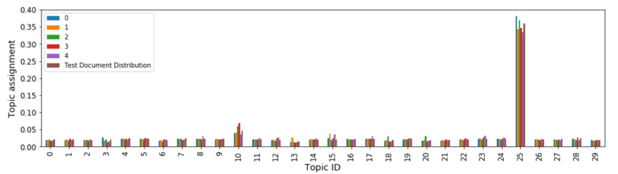
现在,尝试其他一些主题。运行以下代码单元:
plot_topic_distribution(25)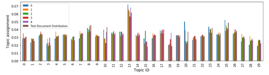
plot_topic_distribution(5000)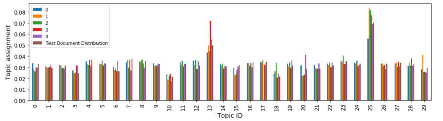
根据您选择的主题数 (NUM_TOPICS),您的绘图可能会略有不同。但总的来说,这些图表明,k-NN 模型使用余弦相似度找到的最近邻文档的主题分布与我们输入模型的测试文档的主题分布非常相似。
结果表明,k-NN 可能是构建基于语义的信息检索系统的好方法,首先将文档嵌入到主题向量中,然后使用 k-NN 模型提供推荐。
总结
恭喜您!在本模块中,您训练、部署并探索了内容推荐模型。
在下一个模块中,您将清理本教程中使用的资源。
清理资源和后续步骤