Amazon SageMaker를 사용한 시멘틱 콘텐츠 추천 시스템 구축

콘텐츠 추천 모델 훈련 및 배포

이 모듈에서는 내장 Amazon SageMaker k-Nearest Neighbors(k-NN) 알고리즘을 사용하여 콘텐츠 추천 모델을 훈련합니다.

Amazon SageMaker k-Nearest Neighbors(k-NN)는 분류 및 회귀 작업을 처리하는 데 사용할 수 있는 인덱스 기반 비모수 지도 학습 알고리즘입니다. 분류 작업의 경우, 이 알고리즘은 타겟에 k개의 최근접 점을 쿼리하여 해당 클래스의 가장 자주 사용되는 레이블을 예측 레이블로 반환합니다. 회귀 문제의 경우, 이 알고리즘은 k 최근접 이웃법에서 반환된 예측 값의 평균을 반환합니다.

k-NN 알고리즘을 사용한 훈련은 샘플링, 차원 축소, 인덱스 작성의 세 단계로 이루어집니다. 샘플링에서는 메모리에 저장될 수 있도록 초기 데이터 세트의 크기를 줄입니다. 차원 축소 단계에서 이 알고리즘은 데이터의 특성 차원을 축소하여 k-NN 모델의 메모리 사용량과 추론 지연 시간을 줄입니다. 랜덤 프로젝션과 빠른 존슨-린든스트라우스 변환이라는 두 가지 차원 축소 방법을 제공합니다. 차원 축소는 차원이 커짐에 따라 희박해지는 데이터의 통계 분석을 어렵게 하는 “차원의 저주”라는 현상을 방지하기 위해 고차원(d >1000) 데이터 세트에 주로 사용합니다. k-NN 훈련의 주 목적은 인덱스를 구성하는 것입니다. 인덱스를 사용하면 추론에 사용할, 값 또는 클래스 레이블이 계산되지 않은 점과 k개의 최근접 점 사이의 거리를 효율적으로 조회할 수 있습니다.

다음 단계에서는 훈련 작업에 사용할 k-NN 알고리즘을 지정하고 모델을 튜닝하기 위한 하이퍼파라미터 값을 설정한 후 모델을 실행합니다. 그런 다음 Amazon SageMaker에서 관리되는 엔드포인트에 모델을 배포하여 예측을 실행합니다.

모듈 완료 시간: 20분

1단계. 훈련 작업 생성 및 실행
1단계. 훈련 작업 생성 및 실행

이전 모듈에서는 주제 벡터를 생성했습니다. 이 모듈에서는 주제 벡터의 인덱스를 유지하는 콘텐츠 추천 모듈을 구축하고 배포합니다.

먼저 셔플링된 레이블을 훈련 데이터의 원래 레이블에 연결하는 사전을 생성합니다. 다음 코드를 복사하여 노트북에 붙여 넣은 다음 [실행]을 선택합니다.
```
labels = newidx 
labeldict = dict(zip(newidx,idx))
```
이제 다음 코드를 사용하여 훈련 데이터를 S3 버킷에 저장합니다.
```
import io
import sagemaker.amazon.common as smac


print('train_features shape = ', predictions.shape)
print('train_labels shape = ', labels.shape)
buf = io.BytesIO()
smac.write_numpy_to_dense_tensor(buf, predictions, labels)
buf.seek(0)

bucket = BUCKET
prefix = PREFIX
key = 'knn/train'
fname = os.path.join(prefix, key)
print(fname)
boto3.resource('s3').Bucket(bucket).Object(fname).upload_fileobj(buf)
s3_train_data = 's3://{}/{}/{}'.format(bucket, prefix, key)
print('uploaded training data location: {}'.format(s3_train_data))
```
다음으로, 다음 헬퍼 함수를 사용하여, 모듈 3에서 생성한 NTM 추정기와 유사한 k-NN 추정기를 생성합니다.
```
def trained_estimator_from_hyperparams(s3_train_data, hyperparams, output_path, s3_test_data=None):
    """
    Create an Estimator from the given hyperparams, fit to training data, 
    and return a deployed predictor
    
    """
    # set up the estimator
    knn = sagemaker.estimator.Estimator(get_image_uri(boto3.Session().region_name, "knn"),
        get_execution_role(),
        train_instance_count=1,
        train_instance_type='ml.c4.xlarge',
        output_path=output_path,
        sagemaker_session=sagemaker.Session())
    knn.set_hyperparameters(**hyperparams)
    
    # train a model. fit_input contains the locations of the train and test data
    fit_input = {'train': s3_train_data}
    knn.fit(fit_input)
    return knn

hyperparams = {
    'feature_dim': predictions.shape[1],
    'k': NUM_NEIGHBORS,
    'sample_size': predictions.shape[0],
    'predictor_type': 'classifier' ,
    'index_metric':'COSINE'
}
output_path = 's3://' + bucket + '/' + prefix + '/knn/output'
knn_estimator = trained_estimator_from_hyperparams(s3_train_data, hyperparams, output_path)
```
훈련 작업이 실행되는 동안 헬퍼 함수의 파라미터를 자세히 살펴봅니다.

Amazon SageMaker k-NN 알고리즘은 최근접 이웃을 계산하기 위한 다양한 거리 지표를 제공합니다. 자연어 처리에 가장 많이 사용되는 지표 중 하나는 코사인 거리입니다. 수학적으로, 벡터 A와 B 사이의 코사인 “유사 계수”는 다음 등식을 사용하여 계산됩니다.

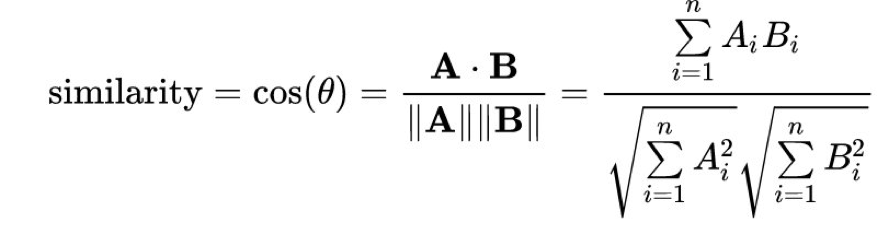
index_metric을 COSINE으로 설정하면 Amazon SageMaker가 자동으로 코사인 유사 계수를 사용하여 최근접 이웃을 계산합니다. 기본 거리는 표준 유클리드 거리인 L2 norm입니다. 게시 당시를 기준으로, COSINE은 faiss.IVFFlat 인덱스 유형에만 지원되고 faiss.IVFPQ 인덱싱 방식에는 지원되지 않습니다.

터미널에 다음 출력이 표시됩니다.
```
Completed - Training job completed
```
성공입니다! 이 모델에서는 특정 테스트 주제가 주어졌을 때 최근접 이웃을 반환하도록 해야 하므로, 라이브 호스팅 엔드포인트로 모델을 배포해야 합니다.

2단계. 콘텐츠 추천 모델 배포

NTM 모델에서와 마찬가지로, k-NN 모델에 대해 다음 헬퍼 함수를 정의하여 엔드포인트를 시작합니다. 이 헬퍼 함수에서 수락 토큰 applications/jsonlines; verbose=true는 최근접 이웃만 반환하는 것이 아니라 모든 코사인 거리를 반환하도록 k-NN 모델에 지시합니다. 추천 엔진을 구축하려면 모델에서 상위 k개의 추천을 구해야 합니다. 그렇게 하려면 verbose 파라미터를 기본값인 false가 아니라 true로 설정해야 합니다.

다음 코드를 복사하여 노트북에 붙여 넣고 [실행]을 선택합니다.

def predictor_from_estimator(knn_estimator, estimator_name, instance_type, endpoint_name=None): 
    knn_predictor = knn_estimator.deploy(initial_instance_count=1, instance_type=instance_type,
                                        endpoint_name=endpoint_name,
                                        accept="application/jsonlines; verbose=true")
    knn_predictor.content_type = 'text/csv'
    knn_predictor.serializer = csv_serializer
    knn_predictor.deserializer = json_deserializer
    return knn_predictor
import time

instance_type = 'ml.m4.xlarge'
model_name = 'knn_%s'% instance_type
endpoint_name = 'knn-ml-m4-xlarge-%s'% (str(time.time()).replace('.','-'))
print('setting up the endpoint..')
knn_predictor = predictor_from_estimator(knn_estimator, model_name, instance_type, endpoint_name=endpoint_name)

다음으로, 추론을 실행할 수 있도록 테스트 데이터를 사전 처리합니다.

다음 코드를 복사하여 노트북에 붙여 넣고 [실행]을 선택합니다.

def preprocess_input(text):
    text = strip_newsgroup_header(text)
    text = strip_newsgroup_quoting(text)
    text = strip_newsgroup_footer(text)
    return text    
    
test_data_prep = []
for i in range(len(newsgroups_test)):
    test_data_prep.append(preprocess_input(newsgroups_test[i]))
test_vectors = vectorizer.fit_transform(test_data_prep)

test_vectors = np.array(test_vectors.todense())
test_topics = []
for vec in test_vectors:
    test_result = ntm_predictor.predict(vec)
    test_topics.append(test_result['predictions'][0]['topic_weights'])

topic_predictions = []
for topic in test_topics:
    result = knn_predictor.predict(topic)
    cur_predictions = np.array([int(result['labels'][i]) for i in range(len(result['labels']))])
    topic_predictions.append(cur_predictions[::-1][:10])

이 모듈의 마지막 단계에서는 콘텐츠 추천 모델을 살펴봅니다.

3단계. 콘텐츠 추천 모델 살펴보기
3단계. 콘텐츠 추천 모델 살펴보기

예측 결과를 얻었으므로 이제 k-NN 모델에서 추천된 k개의 최근접 주제와 비교한 테스트 주제의 주제 분포를 도표로 나타낼 수 있습니다.

다음 코드를 복사하여 노트북에 붙여 넣고 [실행]을 선택합니다.
```
# set your own k.
def plot_topic_distribution(topic_num, k = 5):
    
    closest_topics = [predictions[labeldict[x]] for x in topic_predictions[topic_num][:k]]
    closest_topics.append(np.array(test_topics[topic_num]))
    closest_topics = np.array(closest_topics)
    df = pd.DataFrame(closest_topics.T)
    df.rename(columns ={k:"Test Document Distribution"}, inplace=True)
    fs = 12
    df.plot(kind='bar', figsize=(16,4), fontsize=fs)
    plt.ylabel('Topic assignment', fontsize=fs+2)
    plt.xlabel('Topic ID', fontsize=fs+2)
    plt.show()
```
다음 코드를 실행하여 주제 분포를 도표로 그립니다.
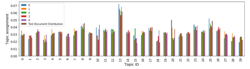
```
plot_topic_distribution(18)
```
이제 다른 주제로 실행해봅니다. 다음 코드 셀을 실행합니다.
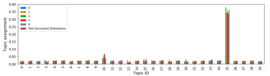
```
plot_topic_distribution(25)
```
```
plot_topic_distribution(5000)
```
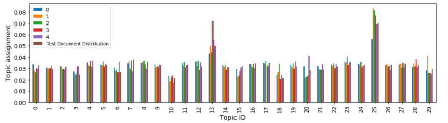
선택하는 주제 수(NUM_TOPICS)에 따라 이 도표와 다르게 나타날 수 있습니다. 하지만 전반적으로, 이러한 도표는 k-NN 모델에서 코사인 유사 계수를 사용해 구한 최근접 이웃 문서의 주제 분포가 모델에 피드로 제공한 테스트 문서와 매우 유사하다는 것을 보여줍니다.

이 결과는 k-NN이 먼저 주제 벡터에 문서를 임베드한 다음 k-NN 모델을 사용하여 추천 서비스를 제공하는 시멘틱 기반 정보 검색 시스템을 구축하는 데 효과적인 방법임을 시사합니다.