Maximize training performance with Gluon data loader workers

With recent advances in CPU and GPU technology, training complex and deep neural network models in a few hours is within reach for many state of-the-art deep models. However, when you use a system with such high processing throughput potential, the required data for the processing pipeline must be ready before each iteration. Any starvation of the processing pipeline results in a direct impact on the performance of the system in terms of system time per epoch. Longer training means slower research advancement and higher costs. So optimization is not only important on systems using GPU, but also on systems using CPU for data processing.

Data pipeline on AWS

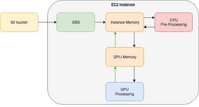
When using Amazon Elastic Compute Cloud (EC2) instances for model training, often the data is warehoused in a Simple Storage Service (S3) bucket. Each EC2 instance is attached to an Amazon Elastic Block Store (EBS) volume, which is used as a local file system. One common data pipeline pattern starts from Amazon S3, goes to Amazon EBS, then to instance memory for pre-processing, and finally to GPU memory for processing.

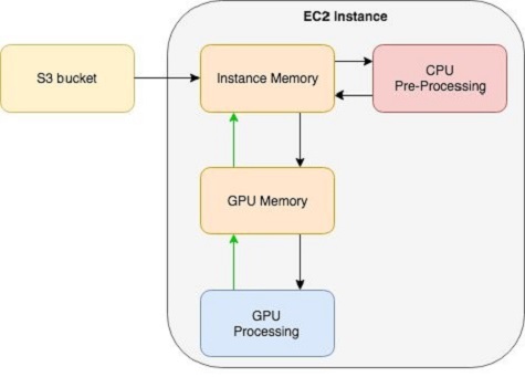
Apache MXNet supports direct connection with Amazon S3, which allows skipping the data transfer from Amazon S3 to Amazon EBS and going directly from Amazon S3 to instance memory for pre-processing, followed by GPU memory for processing. For more information about this feature, refer to this technical note.

For maximizing training performance, the data pipeline must be at least as fast as data processing. The datalink between Amazon S3 and the instance is a network link. Choosing the right instance type can ensure that this connection doesn’t become a bottleneck in the data pipeline. Many EC2 instances support Enhanced Networking with 10 Gigabit or 25 Gigabit network interfaces.

The datalink between EBS and instance memory is moderated by the I/O per second (IOPS) as well as total data bandwidth, between 500 to 4000 Megabit per second throughput depending on the instance type. Using an EBS-Optimized instance can help with ensuring this datalink does not become the bottleneck of the data pipeline. Another technique for increasing the I/O performance is using multiple EBS volumes attached to each EC2 instance. The note on this page contains useful tips on optimizing data loading.

Apache MXNet uses an asynchronous engine to maximize training performance on GPUs by ensuring that data is loaded to GPU memory while computation of the previous batch is in process. To avoid starvation of this high-performance training pipeline, pre-processed data must be available in time for transferring to GPU memory. gluon.data.DataLoader has a built-in mechanism for using workers to address this bottleneck: This is the focus of the rest of this blog post.

gluon.data.DataLoader uses Python’s multiprocessing package to spin up workers to perform data pre-processing in parallel to data processing. Data pre-processing may include data augmentation (e.g., random crop, scale, and mirror in the case of images) and data conditioning (e.g., concatenating different features). In this blog post, I demonstrate how much using workers in gluon.data.DataLoader can impact the system performance.

System configuration

The system I am using in this post is an Amazon EC2 p3.2xlarge instance, but the concept applies to both GPU and multi-core CPU training. I am using MXNet package mxnet_cu90mkl version 1.0.0.post4, installed via pip, which is the latest version of MXNet at the time of this writing. The minimum required MXNet version for this example is version 1.0.0. Instructions on installing MXNet can be found on this page.

I use Deep Learning AMI (Ubuntu) Version 3.0 (ami-0a9fac70) as the Amazon Machine Image (AMI) for my EC2 instance. This AMI is the latest Deep Learning AMI available on AWS Marketplace at the time of the writing. Here is a link for getting started with DLAMI. Alternatively you can use the Amazon SageMaker service, which has MXNet pre-installed.

MNIST example

First, I use a simple convolutional neural network with MNIST dataset to demonstrate the impact of DataLoader workers.

from __future__ import print_function
from time import time
import numpy as np
import mxnet as mx
from mxnet import nd, autograd, gluon
ctx = mx.gpu() if mx.test_utils.list_gpus() else mx.cpu()

Define a convolutional neural network

Now I’ll create a simple 2-layer convolutional network using gluon.nn.

num_fc = 512
num_outputs = 10
net = gluon.nn.HybridSequential()
with net.name_scope():
    net.add(gluon.nn.Conv2D(channels=20, kernel_size=5, activation='relu'))
    net.add(gluon.nn.MaxPool2D(pool_size=2, strides=2))            
    net.add(gluon.nn.Conv2D(channels=50, kernel_size=5, activation='relu'))
    net.add(gluon.nn.MaxPool2D(pool_size=2, strides=2))
    # The Flatten layer collapses all axes, except the first one, into one axis.
    net.add(gluon.nn.Flatten())
    net.add(gluon.nn.Dense(num_fc, activation="relu"))
    net.add(gluon.nn.Dense(num_outputs))

I’ll hybridize the network as well to allow the MXNet engine to perform graph optimization for best performance.

net.hybridize()

I’ll use a softmax cross entropy loss for training.

softmax_cross_entropy = gluon.loss.SoftmaxCrossEntropyLoss()

Write evaluation loop to calculate accuracy

def evaluate_accuracy(data_iterator, net):
    acc = mx.metric.Accuracy()
    for i, (data, label) in enumerate(data_iterator):
        predictions = nd.argmax(net(data.as_in_context(ctx)), axis=1)
        acc.update(preds=predictions, labels=label.as_in_context(ctx))
    return acc.get()[1]

DataLoader and transform function

The transform() function is where data pre-processing happens. In this example, the pre-processing is a simple transpose() operation that reorders the dimensions of the input tensor followed by normalizing to the [0, 1] range. In other applications it can be a complex and processing-intensive operation such as when it’s used for image augmentation.

def transform(data, label):
    return nd.transpose(data.astype(np.float32), (2,0,1))/255, label.astype(np.float32)

def data_loader(train, batch_size, num_workers):
    dataset = gluon.data.vision.MNIST(train=train, transform=transform)
    return gluon.data.DataLoader(dataset, batch_size, shuffle=train, num_workers=num_workers)

Training loop

The training loop is written to be simple and only use a single epoch.

def train(num_workers):
    mx.random.seed(1)
    epochs = 1

    train_data = data_loader(train=True, batch_size=64, num_workers=num_workers)
    test_data = data_loader(train=False, batch_size=64, num_workers=num_workers)

    # Initialize parameters randomly
    net.collect_params().initialize(mx.init.Xavier(magnitude=2.24), ctx=ctx, force_reinit=True)
    trainer = gluon.Trainer(net.collect_params(), 'sgd', {'learning_rate': .1})

    train_start = time()
    for e in range(epochs):
        for data, label in train_data:
            data = data.as_in_context(ctx)
            label = label.as_in_context(ctx)
            # Wait for completion of previous iteration to
            # avoid unnecessary memory allocation
            nd.waitall()
            with autograd.record():
                output = net(data)
                loss = softmax_cross_entropy(output, label)
            loss.backward()
            trainer.step(data.shape[0])
    nd.waitall()
    eval_start = time()
    test_accuracy = evaluate_accuracy(test_data, net)
    eval_end = time()
    print("{} workers: train duration {:.4}, eval duration {:.4}, test accuracy {:.2}".format(
        num_workers, eval_start - train_start, eval_end - eval_start, test_accuracy))

Now we are going to experiment with using different workers for our DataLoader. Note that 0 workers means that the pre-processing step is performed on the main Python process and no worker processes are used to perform pre-processing in parallel. Normally number of workers shouldn’t be increased beyond the number of available CPU cores in the system.

for workers in range(0, 10, 2):
    train(num_workers=workers)

0 workers: train duration 12.96, eval duration 4.154, test accuracy 0.98
2 workers: train duration 6.167, eval duration 2.499, test accuracy 0.98
4 workers: train duration 4.04, eval duration 2.589, test accuracy 0.98
6 workers: train duration 3.765, eval duration 2.61, test accuracy 0.98
8 workers: train duration 3.94, eval duration 2.666, test accuracy 0.98

As you can see from these numbers, increasing the number of workers improves the performance significantly. However after reaching the optimal number of workers, the performance decreases slightly due to the addition of the operating system’s context-switching overhead.

Tips on identifying I/O bottlenecks

A typical symptom of an I/O bottleneck is under-utilization of both GPU and CPU. An easy way to determine if I/O is the bottleneck of the training is to remove any pre-processing of data from the pipeline. If no performance increase is observed, then I/O is the bottleneck.

However, an I/O bottleneck can be both disk I/O or GPU I/O. A GPU I/O bottleneck can be measured by removing disk reads and simply re-loading the same data batch to GPU. If no performance increase is observed, then the system bottleneck is GPU I/O. This means that the training is operating at top performance for the given batch-size, and you can increase the batch size to improve throughput. However if performance increases by removing dependency on disk reads, then disk I/O is the bottleneck. You can use a combination of techniques mentioned earlier to improve the performance of your system.

Conclusion

As I have demonstrated in this blog post, the number of workers can have a dramatic impact on the performance of the system. The optimal number for each setup is completely dependent on the type of pre-processing being performed on the data, as well as the batch size and hardware configuration. After the workers are able to keep up with the processing engine, adding extra workers simply results in a slight reduction in performance due to unnecessary operating system context switches. When starting off with a new training job, feel free to experiment with different numbers of workers and choose the number of workers that provides optimal performance for your experiment. Always choose more workers instead of fewer workers to ensure that the processing engine never starves. Remember to be mindful of potential disk I/O bottlenecks.

About the author

Sina Afrooze is an AWS Software Engineer, focusing on application of Apache MXNet in deep learning for artificial intelligence. His domain expertise is in digital imaging and computer vision.  He enjoys helping AWS customers achieve scale in deep learning solutions using Apache MXNet.