Annotation and segmentation of medical images is a laborious endeavor that can be automated in part via deep learning (DL) techniques. These approaches have achieved state-of-the-art results in generic segmentation tasks, the goal of which is to classify images at the pixel level.

In Part 1 of this blog post, we demonstrate how to train and deploy neural networks to automatically segment brain tissue from an MRI scan in a simple, streamlined way using Amazon SageMaker. We use Apache MXNet to train a convolutional neural network (CNN) on Amazon SageMaker using the Bring Your Own Script paradigm. We train two networks: U-Net and the efficient, low-latency ENet. In Part 2, we will seehow to use AWS Greengrass ML Inference to deploy ENet to a portable edge device for offline inference in low- or no-connectivity environments.

Although the post applies this approach to brain MRIs, as a technique for generic segmentation it’s applicable to similar use cases such as analyzing x-rays.

This blog post provides a high-level overview. For a complete tutorial notebook, see Amazon SageMaker Brain Segmentation on GitHub.

By the end of this blog post, we will predict brain tissue segmentations from MRIs as shown here.

While this use case deals with medical imaging as raw images and not Protected Health Information (PHI), please note the following:

AWS Greengrass is not an AWS HIPAA Eligible Service at the time of this writing. Consistent with the AWS Business Associate Addendum (BAA), AWS Greengrass should not be used to create, receive, maintain, or transmit Protected Health Information (PHI) under the U.S. Health Insurance Portability and Accountability Act (HIPAA). It is each customer’s responsibility to determine whether they are subject to HIPAA, and if so, how best to comply with HIPAA and its implementing regulations. Accounts that create, receive, maintain, or transmit PHI using a HIPAA Eligible Service should encrypt PHI as required under the BAA. For a current list of HIPAA Eligible Services, and for more information generally, see the AWS HIPAA Compliance page.

Overview

Use case

Medical imaging techniques enable medical professionals to see inside the human body, but the professional often needs precise segmentation of the tissues in the image for analytical procedures and inferences. This is particularly relevant in use cases where volumetric and surface analysis are key to deriving insights from the raw images, such as assessing the cardiovascular health of a patient. Typically, medical professionals do this segmentation  manually, which is time-consuming. Recently, convolutional neural networks have been shown to be highly performant at generic segmentation tasks. In this post, we use Amazon SageMaker to train and deploy two such networks to automatically segment brain tissue from MRI images. Amazon SageMaker is a fully managed platform that enables developers and data scientists to quickly and easily build, train, and deploy machine learning (ML) models at any scale.

Of additional interest for such models is edge deployment. Running inference offline at the edge has potential for significant impact in medical image annotation. Given the dearth of medical professionals in parts of the world with limited or no internet connectivity, a portable, low-power solution that can automate annotation locally has many advantages. This post also shows how to deploy models trained in Amazon SageMaker to the edge using AWS Greengrass. This service enables you to run local compute, messaging, data caching, sync, and ML Inference capabilities for connected devices in a secure way.

Setting up

To reproduce the steps outlined here, you need to run the Jupyter notebook with associated code in the repository that accompanies this blog post. Amazon SageMaker provides fully managed instances that are preloaded with ML and DL frameworks and run Jupyter notebooks. We suggest launching one and cloning the repository into your notebook instance to follow along. 

Note – If you do use an Amazon SageMaker notebook instance, you likely need to store the data used in this post on a separate device. Possible choices include using shared memory or mounting an Amazon Elastic File System.

CNN architectures

In this post, we apply two models to the task of brain tissue segmentation:

• U-Net – Introduced in the paper U-Net: Convolutional Networks for Biomedical Image Segmentation, this network was originally used for medical-imaging use cases but has since proven to be reliable in generic segmentation domains. Due to its architectural and conceptual simplicity, it’s often used as a baseline.
• ENet – Introduced in the paper ENet: A Deep Neural Network Architecture for Real-Time Semantic Segmentation, ENet is designed to be low-latency and to operate in environments with low compute capacity (e.g., edge devices). Compared to existing architectures, ENet optimizes for processing time over accuracy.

Data

In this post, we use a small subset of cross-sectional brain MRI data from the Open Access Series of Imaging Studies (OASIS). This project offers a wealth of neuroimaging datasets.

Exploratory data analysis and preprocessing

Before we can start training our networks, we need to visualize the data to better understand it and preprocess it for training a segmentation network. Then we put the preprocessed data on Amazon S3 for Amazon SageMaker to use during model training.

Visualization

The data comes as a vector image in the .img format, each file representing a complete three-dimensional MRI scan of a particular brain. Although organ tissue segmentation is inherently a three-dimensional task, we approximate it by segmenting 2-D cross-sectional MRI slices. This is less complex and compute-intensive than volumetric segmentation and performs reasonably well.

First, load an example into memory as a numpy array and visualize a slice.

image = np.fromfile(
    open(os.path.join(‘example.img'), 'rb'),
    np.dtype('>u2')).reshape((176, 208, 176))

plt.figure(figsize=(12, 12))
plt.title('Input')
plt.imshow(image[:, :, 101], cmap=plt.cm.gray)

The array that we loaded into memory is three-dimensional as expected. We have selected a particular slice along the third axis, as shown in the following image.

As in any semantic segmentation task, the label for each input is a mask of integers, each uniquely corresponding to a particular class. In this case, those classes are types of brain tissue and background, as seen here.

segmentation = np.fromfile(
    open(os.path.join(‘example_mask.img'), 'rb'),
    np.dtype('>u2')).reshape((176, 208, 88))

plt.figure(figsize=(12, 12))
plt.title('Ground Truth')
plt.imshow(segmentation[:, :, 50], cmap=plt.cm.gray)

Preprocessing

Now we need to preprocess the data to train our network on it. We’re going to split the data into a training and validation set (80/20) by patient. This is important to remove any possibility of data leakage; neighboring brain MRI slices will correlate, and splitting by patient ensures clean validation.

train_images, validation_images, train_masks, validation_masks = train_test_split(
    images, masks, test_size=0.2, random_state=1984)

To preprocess the MRI images, we need to convert them from their native format to arrays that we can save as PNG images. The raw MRI arrays have values that represent radiological intensities. These have a far wider range than pixel intensities and are loaded into memory as uint16. Upon saving the slices as PNGs, the data is scaled to fall within the [0,255] range of uint8.

Note – This scaling can result in differences between tissue pixel distributions from image to image, but this doesn’t have an impact on model training.

def process_mris(files, target_dir):
    for f in files:
        mris = np.fromfile(open(f, 'rb'), dtype='>u2')\
            .reshape((176, 208, 176))[:, :, np.arange(1, 176, 2)].transpose((2, 0, 1))
        for i, mri in enumerate(mris):
            new_fname = "_".join(os.path.basename(f).split('.')[0].split('_')[:8])+"_%i.png" % i
            if np.max(mri) <= 255:
                imageio.imsave(os.path.join(
                    target_dir, new_fname), mri.astype(np.uint8))
            else:
                imageio.imsave(os.path.join(target_dir, new_fname), mri)
    return

Notice that we’re grabbing every other slice. This is because the raw MRI is twice as granular as the corresponding mask.

For the masks, we need to save the raw masks as images with exactly one pixel per tissue class. The pixel values of the raw images aren’t exact, and so each raw mask’s pixel values are mapped to a specific integer.

def bin_mask(raw_segmentation):
    raw_segmentation[raw_segmentation <= 150] = 0
    raw_segmentation[np.where((150 < raw_segmentation)
                              & (raw_segmentation <= 400))] = 1
    raw_segmentation[np.where((400 < raw_segmentation)
                              & (raw_segmentation <= 625))] = 2
    raw_segmentation[raw_segmentation > 625] = 3
    return raw_segmentation


def process_labels(files, target_dir):
    for f in files:
        tmp = np.fromfile(open(f, 'rb'), dtype='>u2').reshape(
            (176, 208, 88)).transpose((2, 0, 1))
        masks = bin_mask(tmp)
        for i, mask in enumerate(masks):
            new_fname = "_".join(os.path.basename(f).split(
                '.')[0].split('_')[:8])+"_%i_mask.png" % i
            imageio.imsave(os.path.join(target_dir, new_fname),
                           mask.astype(np.uint8))
    return

Now we can create subsets for test samples and distributed training, compressing each subset.

Model training

Setting up

Begin by importing the Amazon SageMaker Python SDK. We’re going to define the following:

• A session object that provides convenience methods within the context of Amazon SageMaker and our own account.
• An Amazon SageMaker role ARN used to delegate permissions to the training and hosting service. We need this so that these services can access the Amazon S3 buckets where our data and model are stored.

  import sagemaker
  from sagemaker import get_execution_role
  from sagemaker.mxnet import MXNet
  
  sagemaker_session = sagemaker.Session()
  role = get_execution_role()
  

We also imported the Amazon SageMaker estimator object MXNet. This object references default containers that AWS provides, and users provide only entry point scripts and supporting code. Although this tutorial uses the MXNet framework, you can just as easily bring your own script with Tensorflow, Chainer, and now PyTorch.

Uploading data to Amazon S3

Next, upload the preprocessed data to Amazon S3 using the upload_data method to put the objects in a default Amazon SageMaker bucket. Pass the parent directory containing the compressed files to the method, which syncs the child tree to the bucket.

prefix = 'brain-segmentation-tar-gz'
data_bucket = sagemaker_session.upload_data(path=tar_gz_dir, key_prefix=prefix)

Entry Point

As previously mentioned, the MXNet estimator uses a default MXNet container, and the user simply provides the code that defines the training. (For an example, see Training and Hosting SageMaker Models Using the Apache MXNet Module API on GitHub.)

The script that we pass as an entry point to the estimator is brain_segmentation.py.

import os
import tarfile
import mxnet as mx
import numpy as np
from iterator import DataLoaderIter
from losses_and_metrics import avg_dice_coef_metric
from models import build_unet, build_enet
import logging

logging.getLogger().setLevel(logging.DEBUG)

###############################
###     Training Loop       ###
###############################

def train(current_host, channel_input_dirs, hyperparameters, hosts, num_cpus, num_gpus):
    
    logging.info(mx.__version__)
    
    # Set context for compute based on instance environment
    if num_gpus > 0:
        ctx = [mx.gpu(i) for i in range(num_gpus)]
    else:
        ctx = mx.cpu()

    # Set location of key-value store based on training config.
    if len(hosts) == 1:
        kvstore = 'device' if num_gpus > 0 else 'local'
    else:
        kvstore = 'dist_device_sync' if num_gpus > 0 else 'dist_sync'
    
    # Get hyperparameters
    batch_size = hyperparameters.get('batch_size', 16)        
    learning_rate = hyperparameters.get('lr', 1E-3)
    beta1 = hyperparameters.get('beta1', 0.9)
    beta2 = hyperparameters.get('beta2', 0.99)
    epochs = hyperparameters.get('epochs', 100)
    num_workers = hyperparameters.get('num_workers', 6)
    num_classes = hyperparameters.get('num_classes', 4)
    class_weights = hyperparameters.get(
        'class_weights', [[1.35, 17.18, 8.29, 12.42]])
    class_weights = np.array(class_weights)
    network = hyperparameters.get('network', 'unet')
    assert network == 'unet' or network == 'enet', '"network" hyperparameter must be one of ["unet", "enet"]'
    
    # Locate compressed training/validation data
    train_dir = channel_input_dirs['train']
    validation_dir = channel_input_dirs['test']
    train_tars = os.listdir(train_dir)
    validation_tars = os.listdir(validation_dir)
    # Extract compressed image / mask pairs locally
    for train_tar in train_tars:
        with tarfile.open(os.path.join(train_dir, train_tar), 'r:gz') as f:
            f.extractall(train_dir)
    for validation_tar in validation_tars:
        with tarfile.open(os.path.join(validation_dir, validation_tar), 'r:gz') as f:
            f.extractall(validation_dir)
    
    # Define custom iterators on extracted data locations.
    train_iter = DataLoaderIter(
        train_dir,
        num_classes,
        batch_size,
        True,
        num_workers)
    validation_iter = DataLoaderIter(
        validation_dir,
        num_classes,
        batch_size,
        False,
        num_workers)
    
    # Build network symbolic graph
    if network == 'unet':
        sym = build_unet(num_classes, class_weights=class_weights)
    else:
        sym = build_enet(inp_dims=train_iter.provide_data[0][1][1:], num_classes=num_classes, class_weights=class_weights)
    logging.info("Sym loaded")
    
    # Load graph into Module
    net = mx.mod.Module(sym, context=ctx, data_names=('data',), label_names=('label',))
    
    # Initialize Custom Metric
    dice_metric = mx.metric.CustomMetric(feval=avg_dice_coef_metric, allow_extra_outputs=True)
    logging.info("Starting model fit")
    
    # Start training the model
    net.fit(
        train_data=train_iter,
        eval_data=validation_iter,
        eval_metric=dice_metric,
        initializer=mx.initializer.Xavier(magnitude=6),
        optimizer='adam',
        optimizer_params={
            'learning_rate': learning_rate,
            'beta1': beta1,
            'beta2': beta2},
        num_epoch=epochs)
    
    # Save Parameters
    net.save_params('params')
    
    # Build inference-only graphs, set parameters from training models
    if network == 'unet':
        sym = build_unet(num_classes, inference=True)
    else:
        sym = build_enet(
            inp_dims=train_iter.provide_data[0][1][1:], num_classes=num_classes, inference=True)
    net = mx.mod.Module(
        sym, context=ctx, data_names=(
            'data',), label_names=None)
    
    # Re-binding model for a batch-size of one
    net.bind(data_shapes=[('data', (1,) + train_iter.provide_data[0][1][1:])])
    net.load_params('params')
    return net

This script defines the training loop, which constitutes the life cycle of the training job. Some points to notice:

• Hyperparameters – We pass this hyperparameter mapping to the estimator as part of the training configuration.
• Network – This hyperparameter defines the network to train, either unet or enet.
• Local imports – The model, iterator, and loss/metric definitions are in local modules. We pass this script and accompanying modules to the estimator

We encourage you to look at the modules in the tutorial repository to gain deeper insight into these models and iterators.

Note – ML hyperparameter tuning can be complex and time-consuming and require expertise. This is even more true for neural networks. With automatic model tuning in Amazon SageMaker, developers and data scientists can launch hyperparameter tuning jobs that optimize on a given metric or metrics using Bayesian optimization. You can use automatic model tuning on any Amazon SageMaker training job including this one. To see how, we recommend starting with Hyperparameter Tuning with Amazon SageMaker and MXNet on GitHub.

Using local mode for local testing

When bringing your own script or model to Amazon SageMaker, you should test your code to make sure that it’s bug-free. Best practice is to test your custom algorithm container locally.  Otherwise, you have to wait for Amazon SageMaker to spin up your training instance(s) before receiving an error. This is supported with local mode.

To run the container locally, download, install, and configure Docker to run locally with Amazon SageMaker, which you can be do with this helper script.

Next, define the Amazon S3 input types (we test on sample sets).

sample_train_s3 = sagemaker.s3_input(s3_data=os.path.join(
    data_bucket, "sample-train"), distribution='FullyReplicated')
sample_validation_s3 = sagemaker.s3_input(s3_data=os.path.join(
    data_bucket, "sample-validation"), distribution='FullyReplicated')

Now we can define our estimator with training configurations, including the entry point script and directory for the accompanying code. Notice we’re setting train_instance_type to local to launch the job locally.

local_unet_job = 'DEMO-local-unet-job-' + \
    time.strftime("%Y-%m-%d-%H-%M-%S", time.gmtime())

local_estimator = MXNet(entry_point='brain_segmentation.py',
                        base_job_name=local_unet_job,
                        source_dir='source_dir',
                        role=role,
                        train_instance_count=1,
                        train_instance_type='local',
                        hyperparameters={
                            'learning_rate': 1E-3 * 16,
                            'class_weights': [[1.35, 17.18,  8.29, 12.42]],
                            'network': 'unet',
                            'batch_size': 8,
                            'epochs': 1
                        })

Now call fit on the Amazon S3 inputs, mapping train and test labels to each. Because we’re in local mode, the container is downloaded and the image run locally.

local_estimator.fit({'train': sample_train_s3, 'test': sample_validation_s3})

Next, test the serving image locally as well by calling deploy.

local_unet_endpoint = 'DEMO-local-unet-endpoint-' + \
    time.strftime("%Y-%m-%d-%H-%M-%S", time.gmtime())

local_predictor = local_estimator.deploy(initial_instance_count=1, instance_type='local',
                                         endpoint_name=local_unet_endpoint)

The deploy method returns a predictor, which we can use to submit requests to the endpoint.

response = local_predictor.predict(test_brain.tolist())
output = np.argmax(np.array(response), axis=(1))[0].astype(np.uint8)
plt.figure(figsize=(14, 14))
plt.subplot(131)
plt.title('Input')
plt.imshow(test_brain[0][0], cmap=plt.cm.gray)
plt.subplot(132)
plt.title('Ground Truth')
plt.imshow(test_mask[0][0], cmap=plt.cm.gray)
plt.subplot(133)
plt.title('Prediction')
plt.imshow(output, cmap=plt.cm.gray)

At one epoch on a sample data set, the results are predictably terrible, as shown in the following image. Training for more epochs will result in better performance.

Having tested our script, we can launch real training jobs and endpoints with confidence.

U-Net

First, we train U-Net as a baseline for comparison with the faster, lightweight ENet. By default, the training job runs for 100 epochs.

unet_single_machine_job = 'DEMO-unet-single-machine-job-' + \
    time.strftime("%Y-%m-%d-%H-%M-%S", time.gmtime())

unet_single_machine_estimator = MXNet(entry_point='brain_segmentation.py',
                                      base_job_name=unet_single_machine_job,
                                      source_dir='source_dir',
                                      role=role,
                                      train_instance_count=1,
                                      train_instance_type='ml.p3.2xlarge',
                                      hyperparameters={
                                          'learning_rate': 1E-3,
                                          'class_weights': [[1.35, 17.18,  8.29, 12.42]],
                                          'network': 'unet',
                                          'batch_size': 32,
                                      })

This time, train on the entire training set and validate on the entire validation set.

train_s3 = sagemaker.s3_input(s3_data=os.path.join(
    data_bucket, "train"), distribution='FullyReplicated')
validation_s3 = sagemaker.s3_input(s3_data=os.path.join(
    data_bucket, "validation"), distribution='FullyReplicated')

unet_single_machine_estimator.fit({'train': train_s3, 'test': validation_s3})

ENet

To train ENet, just change the network hyperparameter to enet.

enet_single_machine_job = 'DEMO-enet-single-machine-job-' + \
    time.strftime("%Y-%m-%d-%H-%M-%S", time.gmtime())

enet_single_machine_estimator = MXNet(entry_point='brain_segmentation.py',
                                      base_job_name=enet_single_machine_job,
                                      source_dir='source_dir',
                                      role=role,
                                      train_instance_count=1,
                                      train_instance_type='ml.p3.2xlarge',
                                      hyperparameters={
                                          'learning_rate': 1E-3,
                                          'class_weights': [[1.35, 17.18,  8.29, 12.42]],
                                          'network': 'enet',
                                          'batch_size': 32,
                                      })

enet_single_machine_estimator.fit({'train': train_s3, 'test': validation_s3})

Distributed training

The data that we have trained on is a very small subset of what’s available at OASIS. With training at scale, distributed training is often a more cost-effective approach to training your network than vertical scaling, in terms of both time and money. At our scale, this approach might or might not be faster than a single machine, but we provide it as demonstration.

Launching a distributed training job on Amazon SageMaker with your own script takes only a few steps, as follows:

• The script that we provide must support distributed training. In MXNet, do this by defining a key-value store. This portion of the entry point script checks to see if the job has multiple devices and, if so, defines the key-value store for synchronous distributed training.

  if len(hosts) == 1:
          kvstore = 'device' if num_gpus > 0 else 'local'
      else :
          kvstore = 'dist_device_sync' if num_gpus > 0 else 'dist_sync'

• Set train_instance_count from one to many.
• Shard training data across nodes.

For the last step, we define a sharded Amazon S3 input by setting distribution to ShardedByS3Key. This option attempts to evenly split the number of objects under the provided prefix across nodes (this implicitly means you need as many objects under the prefix as nodes). Had you kept this argument as FullyReplicated, each node would have copies of the entire data set.

distributed_train_s3 = sagemaker.s3_input(s3_data=os.path.join(
    data_bucket, "dist"), distribution='ShardedByS3Key')

Now you can launch a distributed training job.

unet_distributed_job = 'DEMO-unet-distributed-job-' + \
    time.strftime("%Y-%m-%d-%H-%M-%S", time.gmtime())

unet_distributed_estimator = MXNet(entry_point='brain_segmentation.py',
                                   base_job_name=unet_distributed_job,
                                   source_dir='source_dir',
                                   role=role,
                                   train_instance_count=2,
                                   train_instance_type='ml.p3.2xlarge',
                                   hyperparameters={
                                       'epochs': 50,
                                       'learning_rate': 1E-3,
                                       'class_weights': [[1.35, 17.18,  8.29, 12.42]],
                                       'network': 'unet',
                                       'batch_size': 32,
                                   })

unet_distributed_estimator.fit({'train': distributed_train_s3,
                                'test': validation_s3})

Deploying the inference endpoints

Now that we’ve trained both models, we can use Amazon SageMaker to deploy them to web-hosted HTTP endpoints to serve inferences and predictions at low latency. By default, these endpoints respond to POST requests of in-memory image arrays.

Deploying the U-Net endpoint

First we deploy U-Net to an endpoint.

unet_endpoint = 'DEMO-unet-endpoint-' + \
    time.strftime("%Y-%m-%d-%H-%M-%S", time.gmtime())

unet_predictor = unet_single_machine_estimator.deploy(instance_type='ml.c5.xlarge', 
initial_instance_count=1, endpoint_name=unet_endpoint)

Let’s get a test response and compare the inference with the input and ground truth.

response = unet_predictor.predict(test_brain.tolist())
output = np.argmax(np.array(response), axis=(1))[0].astype(np.uint8)
plt.figure(figsize=(14, 14))
plt.subplot(131)
plt.title('Input')
plt.imshow(test_brain[0][0], cmap=plt.cm.gray)
plt.subplot(132)
plt.title('Ground Truth')
plt.imshow(test_mask[0][0], cmap=plt.cm.gray)
plt.subplot(133)
plt.title('Prediction')
plt.imshow(output, cmap=plt.cm.gray)

Qualitatively speaking, these results in the following image look promising.

Deploying the ENet endpoint

Now let’s deploy our ENet model. Instead of using the deploy method in estimator, as an exercise we create a model object, MXNetModel, instead. We pass the location of the ENet model artifact from the training job. This is how you would bring your own model to Amazon SageMaker to deploy to an endpoint.

enet_endpoint = 'DEMO-enet-endpoint-' + \
    time.strftime("%Y-%m-%d-%H-%M-%S", time.gmtime())
enet_model = sagemaker.mxnet.MXNetModel(enet_single_machine_estimator.model_data, role, 
'brain_segmentation.py', source_dir='source_dir', framework_version="1.0")

enet_predictor = enet_model.deploy(
    instance_type='ml.c5.xlarge', initial_instance_count=1)

Let’s get a test response and compare the inference with the input and ground truth.

response = enet_predictor.predict(test_brain.tolist())
output = np.argmax(np.array(response), axis=(1))[0].astype(np.uint8)
plt.figure(figsize=(14, 14))
plt.subplot(131)
plt.title('Input')
plt.imshow(test_brain[0][0], cmap=plt.cm.gray)
plt.subplot(132)
plt.title('Ground Truth')
plt.imshow(test_mask[0][0], cmap=plt.cm.gray)
plt.subplot(133)
plt.title('Prediction')
plt.imshow(output, cmap=plt.cm.gray)

Again, the results in the following image look qualitatively promising.

Invoking the endpoint using an Amazon S3 URI

MXNet endpoints in Amazon SageMaker are by default set up to run inference on data sent via POST request. The assumption is that the data sent is in the format of the data that the model is trained on. For computer vision models, this can be problematic due to the bandwidth limits on Amazon SageMaker requests.

One workaround is to instead submit an Amazon S3 Uniform Resource Identifier (URI), have the endpoint download the image locally, transform, and put the resulting mask back to Amazon S3. In this approach, there is no limit to the size of the content transformed.

Let’s take a look at what entry point for this custom serving image would look like.

from __future__ import absolute_import
import boto3
import base64
import json
import io
import os
import mxnet as mx
from mxnet import nd
import numpy as np
mx.test_utils.download("https://s3.amazonaws.com/sagemaker-png/png.py", "png.py")
import png

###############################
###     Hosting Code        ###
###############################

def push_to_s3(img, bucket, prefix):
    """
    A method for encoding an image array as png and pushing to Amazon S3

    Parameters
    ----------
    img : np.array
        Integer array representing image to be uploaded.
    bucket : str
        S3 Bucket to upload to.
    prefix : str
        Prefix to upload encoded image to (should be .png).
    """
    s3 = boto3.client('s3')
    png.from_array(img.astype(np.uint8), 'L').save('img.png')
    response = s3.put_object(
        Body=open('img.png', 'rb'),
        Bucket=bucket,
        Key=prefix
    )
    return

def download_from_s3(bucket, prefix):
    """
    A method for downloading object from Amazon S3

    Parameters
    ----------
    bucket : str
        Amazon S3 bucket to download from.
    prefix : str
        Prefix to download from.
    """
    s3 = boto3.client('s3')
    response = s3.get_object(Bucket=bucket, Key=prefix)
    return response

def decode_response(response):
    """
    A method decoding raw image bytes from Amazon S3 call into mx.ndarray.

    Parameters
    ----------
    response : dict
        Dict of Amazon S3 get_object response.
    """
    data = response['Body'].read()
    b64_bytes = base64.b64encode(data)
    b64_string = b64_bytes.decode()
    return mx.image.imdecode(base64.b64decode(b64_string)).astype(np.float32)

def transform_fn(net, data, input_content_type, output_content_type):
    try:
        inp = json.loads(json.loads(data)[0])
        bucket = inp['bucket']
        prefix = inp['prefix']
        s3_response = download_from_s3(bucket, prefix)
        img = decode_response(s3_response)
        img = nd.expand_dims(nd.transpose(img, (2, 0, 1)), 0)
        img = nd.sum_axis(nd.array([[[[0.3]], [[0.59]], [[0.11]]]]) * img, 1, keepdims=True)
        batch = mx.io.DataBatch([img])
        net.forward(batch)
        raw_output = net.get_outputs()[0].asnumpy()
        mask = np.argmax(raw_output, axis=(1))[0].astype(np.uint8)
        output_prefix = os.path.join(
            'output', '/'.join(prefix.split('/')[1:]).split('.')[0] + '_MASK_PREDICTION.png')
        push_to_s3(mask, bucket, output_prefix)
        response = {'bucket': bucket, 'prefix': output_prefix}
    except Exception as e:
        response = {'Error': str(e)}
    return json.dumps(response), output_content_type

Because we already have a trained model, we directly define the model object using MXNetModel with the Amazon S3 location of our model artifact from the earlier training job.

unet_s3_endpoint = 'DEMO-unet-s3-endpoint-' + \
    time.strftime("%Y-%m-%d-%H-%M-%S", time.gmtime())

unet_s3_model = sagemaker.mxnet.MXNetModel(unet_single_machine_estimator.model_data, role,
                                           entry_point="brain_segmentation_s3_transform.py", source_dir='source_dir')

unet_s3_predictor = unet_s3_model.deploy(instance_type='ml.c5.xlarge', initial_instance_count=1,
                                         endpoint_name=unet_s3_endpoint)

Now we upload our test image to Amazon S3.

s3 = boto3.client('s3')
test_bucket = "<YOUR-BUCKET-HERE>"
prefix = "test_img.png"
s3.upload_file(Filename=os.path.join(‘test.png'),
               Bucket=test_bucket, Key=prefix)

The body of our request will be in JSON format, so define a dict containing the relevant fields and invoke the endpoint.

request_body = json.dumps({"bucket": test_bucket, "prefix": prefix})

response = unet_s3_predictor.predict([request_body])

Now download the result and visualize.

s3.download_file(Bucket=response['bucket'],
                 Key=response['prefix'], Filename="result.png")

plt.figure(figsize=(14, 14))
plt.subplot(131)
plt.title('Input')
plt.imshow(test_brain[0][0], cmap=plt.cm.gray)
plt.subplot(132)
plt.title('Ground Truth')
plt.imshow(test_mask[0][0], cmap=plt.cm.gray)
plt.subplot(133)
plt.title('Prediction')
plt.imshow(np.array(Image.open("result.png")), cmap=plt.cm.gray)

Evaluating and comparing the models

Both models look qualitatively performant, but we need to quantify this and compare the latency between the two models. Recall that ENet is designed to trade off accuracy for efficiency and low latency.

Using confusion matrices

An effective way to visualize performance for multi-class classification is with a confusion matrix, which compares ground truth labels with predicted labels. Because semantic segmentation is ostensibly per-pixel multiclass classification, confusion matrices are useful here, too.

We use the following code from the scikit-learn documentation to plot confusion matrices.

from sklearn.metrics import confusion_matrix
import itertools


def plot_confusion_matrix(cm, classes,
                          normalize=False,
                          title='Confusion matrix',
                          cmap=plt.cm.Blues):
    """
    This function prints and plots the confusion matrix.
    Normalization can be applied by setting `normalize=True`.
    """
    if normalize:
        cm = cm.astype('float') / cm.sum(axis=1)[:, np.newaxis]
        print("Normalized confusion matrix")
    else:
        print('Confusion matrix, without normalization')

    print(cm)

    plt.imshow(cm, interpolation='nearest', cmap=cmap)
    plt.title(title)
    plt.colorbar()
    tick_marks = np.arange(len(classes))
    plt.xticks(tick_marks, classes, rotation=45)
    plt.yticks(tick_marks, classes)

    fmt = '.2f' if normalize else 'd'
    thresh = cm.max() / 2.
    for i, j in itertools.product(range(cm.shape[0]), range(cm.shape[1])):
        plt.text(j, i, format(cm[i, j], fmt),
                 horizontalalignment="center",
                 color="white" if cm[i, j] > thresh else "black")

    plt.tight_layout()
    plt.ylabel('True label')
    plt.xlabel('Predicted label')

#Citations
#@article{scikit-learn,
# title={Scikit-learn: Machine Learning in {P}ython},
# author={Pedregosa, F. and Varoquaux, G. and Gramfort, A. and Michel, V.
#         and Thirion, B. and Grisel, O. and Blondel, M. and Prettenhofer, P.
#         and Weiss, R. and Dubourg, V. and Vanderplas, J. and Passos, A. and
#         Cournapeau, D. and Brucher, M. and Perrot, M. and Duchesnay, E.},
# journal={Journal of Machine Learning Research},
# volume={12},
# pages={2825--2830},
# year={2011}
#}

We can use the U-Net endpoint to get predictions to compare to ground truths from the validation set.

ground_truths = []
outputs = []
for validation_pair in validation_pairs:
    img = np.array(Image.open(os.path.join(validation_dir, validation_pair[0])))[
        np.newaxis, np.newaxis, :]
    response = unet_predictor.predict(img.tolist())
    outputs.append(np.argmax(np.array(response), axis=(1))[0].astype(np.uint8))
    ground_truths.append(
        np.array(Image.open(os.path.join(validation_dir, validation_pair[1]))))
ground_truths = np.concatenate(ground_truths)
outputs = np.concatenate(outputs)
ground_truths = ground_truths.flatten()
outputs = outputs.flatten()

Now we can compare the predictions to the ground truth labels.

# Compute confusion matrix
cnf_matrix = confusion_matrix(ground_truths, outputs)
np.set_printoptions(precision=2)
class_names = [0, 1, 2, 3]

# Plot non-normalized confusion matrix
plt.figure()
plot_confusion_matrix(cnf_matrix, classes=class_names,
                      title='Confusion matrix, without normalization')

# Plot normalized confusion matrix
plt.figure()
plot_confusion_matrix(cnf_matrix, classes=class_names, normalize=True,
                      title='Normalized confusion matrix')

plt.show()

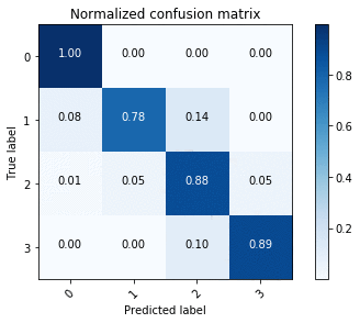
This gives us the normalized confusion matrix, as shown in the following image.

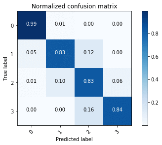
Doing the same with the ENet endpoint provides the confusion matrix in the following image.

Using the confusion matrices, we see that U-Net outperforms ENet in terms of accuracy overall, but this is to be expected given the accuracy-latency tradeoff.

Quantifying inference latency

To quantify inference times for the two models, we timed forward passes for U-Net and ENet in the following environments:

• Amazon EC2 c5.2xlarge instances for CPU with MKL-DNN
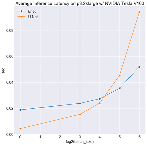
• Amazon EC2 p3.2xlarge instances for GPU with NVIDIA Tesla V100
• Raspberry Pi 3 (RPi) board

We ran trials for batch sizes of 1, 8, 16, 32, and 64.

Results for the CPU environment

As shown in the following image, at all batch sizes, ENet runs faster than U-Net and is real-time. ENet is designed to require 75 times less FLOPS than models like U-Net, and the effect on latency is apparent.

Results for the GPU environment

Interestingly, U-Net is faster than ENet at smaller batch sizes, as shown in the following image.

This might seem counterintuitive, but it makes sense when you consider the respective sizes of each network’s symbolic graph. Symbolically ENet is considerably larger than U-Net (see here), which translates to more kernel launches upon inference. At smaller batch sizes, the cost of launching kernels and transferring memory outweighs ENet’s computational gains, and it’s slower. At a certain threshold, the computational efficiency overtakes this cost, and it’s faster than U-Net.

You could ameliorate this by optimizing ENet’s computational graph through NVIDIA TensorRT, which among other things provides kernel fusion. This technique fuses layers and tensors to ensure that each kernel launch maximizes computation. It’s coming soon to MXNet.

Results for the RPi (CPU) environment

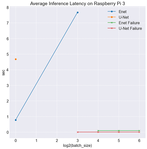
Based on results from benchmarking on CPU, we expect ENet to outperform U-Net on RPi, and that is indeed the case, as shown in the following image.

What’s more important is how ENet is effective in a low-resource environment. At batch sizes 16, 32, and 64, the RPi was unable to hold the test data in memory. However, at batch size 8, U-Net failed, and ENet didn’t. This is a testament to ENet’s low impact because the RPi board couldn’t handle U-Net inference for the same batch size. Enet is also low impact in terms of model size, with 1.5 Mb worth of parameters compared to U-Net’s 30 Mb, making it ideal for edge inference.

Conclusion

In Part 1 of this post, we have shown how to train a convolutional neural network to automate brain tissue segmentation by bringing your own MXNet script to Amazon SageMaker. We showed how to test your script locally using local mode and how to shard your data for distributed training jobs. Aside from default endpoint deployment, we demonstrated how you can write custom serving code to respond to Amazon S3 URIs instead of image data. We discussed the tradeoff of accuracy and efficiency between U-Net and ENet, and we determined that ENet is ideal in low-resource environments.

In Part 2, we see how to use AWS Greengrass to deploy our ENet model trained in Amazon SageMaker to an edge device. There it serves inference as a portable ML solution for brain segmentation.

Acknowledgements

This work was made possible with data provided by Open Access Series of Imaging Studies (OASIS), OASIS-1, by Marcus et al., 2007, used under CC BY 4.0.

The following data were provided by OASIS:

• OASIS-3: Principal Investigators: T. Benzinger, D. Marcus, J. Morris; NIH P50AG00561, P30NS09857781, P01AG026276, P01AG003991, R01AG043434, UL1TR000448, R01EB009352. AV-45 doses were provided by Avid Radiopharmaceuticals, a wholly owned subsidiary of Eli Lilly.
• OASIS: Cross-Sectional: Principal Investigators: D. Marcus, R, Buckner, J, Csernansky J. Morris; P50 AG05681, P01 AG03991, P01 AG026276, R01 AG021910, P20 MH071616, U24 RR021382.
• OASIS: Longitudinal: Principal Investigators: D. Marcus, R, Buckner, J. Csernansky, J. Morris; P50 AG05681, P01 AG03991, P01 AG026276, R01 AG021910, P20 MH071616, U24 RR021382.

Publications:

• Open Access Series of Imaging Studies (OASIS): Cross-Sectional MRI Data in Young, Middle Aged, Nondemented, and Demented Older Adults

Marcus, DS, Wang, TH, Parker, J, Csernansky, JG, Morris, JC, Buckner, RL. Journal of Cognitive Neuroscience, 19, 1498-1507. doi: 10.1162/jocn.2007.19.9.1498

About the Author

Brad Kenstler is a Data Scientist on the Amazon Machine Learning Solutions Lab team. As part of the ML Solutions Lab, he helps AWS customers leverage ML & AI within their own organization for their own business use-cases and processes. His primary field of interest lies in the intersection of computer vision and deep learning. Outside of work, Brad enjoys listening to heavy metal, tasting new bourbons, and watching the San Francisco 49ers.
.