Artificial Intelligence
Choose the best AI accelerator and model compilation for computer vision inference with Amazon SageMaker
AWS customers are increasingly building applications that are enhanced with predictions from computer vision models. For example, a fitness application monitors the body posture of users while exercising in front of a camera and provides live feedback to the users as well as periodic insights. Similarly, an inventory inspection tool in a large warehouse captures and processes millions of images across the network, and identifies misplaced inventory.
After a model is trained, machine learning (ML) teams can take up to weeks to choose the right hardware and software configurations to deploy the model to production. There are several choices to make, including the compute instance type, AI accelerators, model serving stacks, container parameters, model compilation, and model optimization. These choices are dependent on application performance requirements like throughput and latency as well as cost constraints. Depending on the use case, ML teams need to optimize for low response latency, high cost-efficiency, high resource utilization, or a combination of these given certain constraints. To find the best price/performance, ML teams need to tune and load test various combinations and prepare benchmarks that are comparable for a given input payload and model output payload.
Amazon SageMaker helps data scientists and developers prepare, build, train, and deploy high-quality ML models quickly by bringing together a broad set of capabilities purpose built for ML. SageMaker provides state-of-the-art open-source model serving containers for XGBoost (container, SDK), scikit-learn (container, SDK), PyTorch (container, SDK), TensorFlow (container, SDK), and Apache MXNet (container, SDK). SageMaker provides three options to deploy trained ML models for generating inferences on new data. Real-time inference endpoints are suitable for workloads that need to be processed with low latency requirements. There are several instances to choose from, including compute-optimized, memory-optimized, and AI accelerators like AWS Inferentia for inference with SageMaker. Amazon SageMaker Neo is a capability of SageMaker that automatically compiles Gluon, Keras, MXNet, PyTorch, TensorFlow, TensorFlow-Lite, and ONNX models for inference on a range of target hardware.
In this post, we show how to set up a load test benchmark for a PyTorch ResNet50 image classification model with the SageMaker pre-built TorchServe container and a combination of instance choices like g4dn with Nvidia T4 GPU and Inf1 with AWS Inferentia, as well as model compilation with Neo.
The following posts are relevant to this topic:
- A complete guide to AI accelerators for deep learning inference — GPUs, AWS Inferentia and Amazon Elastic Inference – The author describes how to choose the right AI accelerator for inference on AWS. The compute choices include CPUs and a range of NVIDIA GPUs like NVIDIA T4 and AWS Inferentia.
- Maximize TensorFlow performance on Amazon SageMaker endpoints for real-time inference – The performance tuning described in this post includes selecting model and container parameters for high peak throughput and low latency.
- Speed up YOLOv4 inference to twice as fast on Amazon SageMaker – The model in this post is compiled with Neo and compared against an uncompiled model on the same instance.
- Achieving 1.85x higher performance for deep learning based object detection with an AWS Neuron compiled YOLOv4 model on AWS Inferentia – The author describes how to achieve higher performance for a TensorFlow YOLOv4 model on AWS Inferentia based Amazon EC2 Inf1 instances. This model is compiled with AWS Neuron and compared against an uncompiled model on a g4dn Amazon Elastic Compute Cloud (Amazon EC2) instance.
Experiment overview
In this post, we set up concurrent client connections to increase the load up to peak throughput per second (TPS). We demonstrate that for this image classification CV task, AWS Inferentia instances are 5.4 times more price performant than g4dn instances with a compiled model. A model compiled with Neo and deployed to a g4dn instance results in 1.9 times higher throughput, 50% lower latency, and 50% lower cost per 1 million inferences than a model deployed to the same instance without compilation. Additionally, a model compiled with Neo and deployed to an Inf1 instance results in 4.1 times higher throughput, 77% lower latency, and 90% lower cost per 1 million inferences than a model deployed to a g4dn instance without compilation.
The following diagram illustrates the architecture of our experiment.
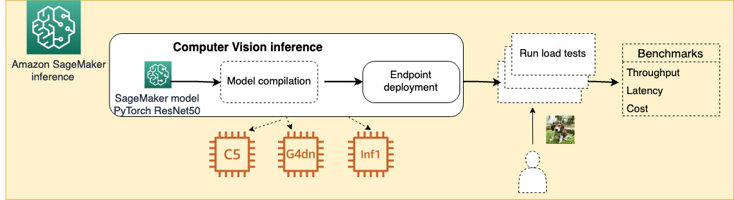
The code used for this experiment is included in the GitHub repo.
AI accelerators and model compilation
In our tests, we deploy and test the performances of a pre-trained ResNet50 model from the PyTorch Hub. The model is deployed on three different instances:
- For the CPU instances, we choose c5.xlarge. This instance offers a first or second-generation Intel Xeon Platinum 8000 series processor (Skylake-SP or Cascade Lake) with a sustained all core Turbo CPU clock speed of up to 3.6 GHz.
- For the GPU instances, we choose g4dn.xlarge. These instances are equipped with NVIDIA T4 GPUs, which deliver up to 40 times better low latency throughput than CPUs, making them the most cost-effective for ML inference.
- We test the two against the AWS Inferentia instances, with the inf1.xlarge instance. Inf1 instances are built from the ground up to support ML inference applications: they deliver up to 2.3 times higher throughput and up to 70% lower cost per inference than comparable current generation GPU-based EC2 instances.
We also compile the models with Neo and compare the performances of the standard model versus its compiled form.
The model
ResNet50 is a variant of the ResNet model, which has 48 convolution layers along with one MaxPool and one average pool layer. It has 3.8 x 10^9 floating point operations (FLOPS). ResNets were introduced in 2015 with the paper “Deep Residual Learning for Image Recognition” (ArXiv) and have been used ever since; they provide state-of-the-art results for many classification and detection tasks.
The variant that we use is the PyTorch implementation. Its documentation is available on its PyTorch Hub page, and it comes pre-trained on the ImageNet dataset.
The payload
To test our model, we use a 3x224x224 JPG image of a beagle puppy sitting on grass, found on Wikimedia.

This image is passed as bytes in the body of the request to the SageMaker endpoint. The image size is 21 KB. The endpoint is responsible of reading the bytes, parsing it to pytorch.Tensor, then doing a forward pass with the model.
Run the experiment
We start by launching an Amazon SageMaker Studio notebook on an ml.c5.4xlarge instance. This is our main instance to download the model, deploy it to SageMaker real-time instances, and test latency and throughput. Studio notebooks are optional in reproducing the results of this experiment, because you could also use SageMaker notebook instances, other cloud services for compute such as AWS Lambda, Amazon EC2, or Amazon Elastic Container Service (Amazon ECS), or your local IDE of choice. In this post, we assume that you already have a Studio domain up and running. If that’s not the case, you can onboard Studio.
After you open your Studio domain, you can clone the repository available on GitHub, and open the resnet50.ipynb notebook. You can switch the underlying instance by choosing the details (see the following screenshot), choosing ml.c5.4xlarge, then switching the kernel to the Python 3 (PyTorch 1.6 Python 3.6 CPU Optimized) option.

The process to spin up the new instance and attach the kernel takes approximately 3–4 minutes. When it’s complete, you can run the first cell, which is responsible for downloading the model locally before uploading it to Amazon Simple Storage Service (Amazon S3). This cell uses the default bucket for SageMaker as the S3 bucket of choice, and the prefix that you provide. The following is the default code:
If you leave the download_the_model parameter set to False, you don’t download the model. This is ideal if you plan on running the notebook again in the same account.
For SageMaker to deploy the model to a real-time endpoint, SageMaker needs to know which container image is responsible for hosting the model. The SageMaker Python SDK provides some abstractions to simplify our job here, because the best-known frameworks are supported natively. For this post, we use an object called PyTorchModel, which provides the correct image URI given the framework version and creates the abstraction of the model that we use for deployment. For more information about how SageMaker deploys the PyTorch model server, see The SageMaker PyTorch Model Server. Our PyTorchModel is instantiated with the following code:
Let’s deep dive into the parameters:
- model_data – Represents the S3 path containing the
.tar.gzfile with the model. - entry_point – This Python script contains the inference logic, how to load the model (
model_fn), how to preprocess the data before inference (input_fn), how to perform inference (predict_fn), and how to postprocess the data after inference (output_fn). For more details, see The SageMaker PyTorch Model Server. - source_dir – The folder containing the entry point file, as well as other useful files, such as other dependencies and the
requirements.txtfile. - framework_version and py_version – The version of Python and PyTorch that we want to use.
- role – The role to assign to the endpoint to access the different AWS resources.
After we set up our model object, we can deploy it to a real-time endpoint. The SageMaker Python SDK makes it easy for us to do this, because we only need one function: model.deploy(). This function accepts two parameters:
- initial_instance_count – How many instances we should use for the real-time endpoint initially, after which it can auto scale if configured to do so. For more information, see Automatically Scale Amazon SageMaker Models.
- instance_type – The instance to use for deployment.
As stated previously, we deploy the model as is to a managed SageMaker endpoint with a CPU instance (ml.c5.xlarge) and to a GPU-equipped managed SageMaker instance (ml.g4dn.xlarge). Now that the model has been deployed, we can test it. This is made possible either by the Python SDK for SageMaker and its method predict(), or via the Boto3 client defined in the AWS SDK for Python and its method invoke_endpoint(). At this step, we don’t try to run a prediction with either of the APIs. Instead, we store the endpoint name to use it later in our tests battery.
Compile the model with Neo
A common tactic in more advanced use cases is to improve model performance, in terms of latency and throughput, by compiling the model. SageMaker features its own compiler, Neo, which enables data scientists to optimize ML models for inference on SageMaker in the cloud and supported devices at the edge.
We need to complete a few steps to make sure that the model can be compiled. First of all, make sure that the model you’re trying to compile and its framework are supported by the Neo compiler. Because we’re deploying on instances managed by SageMaker, we can refer to the following list of supported instance types and frameworks. Our ResNet50 with PyTorch 1.6 is among the supported ones, so we can proceed.
The next step is to prepare the model for compilation. Neo requires that models satisfy specific input data shapes, and models are saved according to a specific data structure. According to the PyTorch model directory structure, the contents of the model.tar.gz file should have the model itself be at the root of the file, and the inference code under the code/ folder. We use the tarfile package in Python to create the archive file in the following way:
Next, we upload the file to Amazon S3. Then we can compile it by instantiating a new PyTorchModel object, then call the compile() function. This function expects a few parameters:
- target_instance_family – The target instance of your compilation. For a list of valid values, see TargetDevice.
- input_shape – The input shape expected by the model, as set during model save.
- output_path – Where to store the output of your compilation job (the compiled model).
Compilation starts by running the following code snippet:
Compile for AWS Inferentia instances
We can try one more thing to improve our model performance: use AWS Inferentia instances. AWS Inferentia instances require the model to be compiled with the Neuron SDK, which is already part of the Neo compiler, when choosing ml_inf1 as the target of the compilation. To know which deep learning frameworks and models are supported by AWS Inferentia with SageMaker, see AWS Inferentia. You can also learn more about the Neuron SDK on the service page and developer documentation. We compile and deploy for AWS Inferentia instances by running the following code:
Experiment results
To measure throughput and latency, we have written a test script that is available in the repository in the load_test.py file. The load test module creates multiple concurrent client invocations with Python multi-threading and measures the throughput per second and end-to-end latency. In our tests, we chose ml.c5.4xlarge as our client test instance and configured the test script to use 16 concurrent threads (num_threads=16) because the instance comes with 16 vCPUs. For more information about the instance specifications, see Amazon SageMaker Pricing. Furthermore, our tests only use one image per inference. Batching of multiple images per inference brings different results for all of the following instances. The results are reported in the following table.

Although throughput and latency are two measures that are already good enough to define the best performing instance/compilation combination, they don’t take into account the hourly cost of the instances. To do so, we showcase a popular metric for inference, the cost per 1 million inferences. The following plots summarize the results obtained in our tests: AWS Inferentia machines are the most cost-effective instances for CV inference workloads, with $0.3 per 1 million inferences compared to $1.62 of the compiled model on the g4dn.xlarge instance and $4.95 of the compiled model on the ml.c5.xlarge instance, making inf1.xlarge instances respectively 5.4 times and 16.5 times more cost-effective.

When we take into account the sheer number of transactions per hour (TPH), AWS Inferentia instances also show the best performance, achieving 1.1 million TPH, compared to 0.5 million TPH of the GPU-compiled model and the 40,000 TPH of the CPU-compiled model.

Conclusion
In this post, we used a pre-trained ResNet50 model from the PyTorch Vision Hub, deployed it with SageMaker on multiple instance types, and load tested the performance before and after compilation. The models were deployed on instances with different AI accelerators for inference, namely CPU (ml.c5.xlarge), GPU (ml.g4dn.xlarge), and AWS Inferentia chips (ml.inf1.xlarge). Tests conducted by concurrent invocations of the model with one input image of shape 3x224x224 showed that AWS Inferentia instances had the highest throughput per second (304.3 inferences per second), the lowest latency (4.9 milliseconds), and the highest cost-efficiency ($0.30$ per 1 million inferences).
These results demonstrate that AWS Inferentia instances provide the highest price/performance for CV workloads on SageMaker. You can check your model compatibility with AWS Inferentia by reviewing the supported operators for PyTorch and TensorFlow. Neo provides model compilation for models to be deployed with AWS Inferentia as well as general-purpose GPU instances. Models that aren’t yet supported with AWS Inferentia instances can be compiled with Neo and deployed to GPU instances for a two-fold improvement in both TPS and latency as compared to direct deployment.
You can also try out other model optimization techniques like distillation, pruning, and quantization. Use the benchmarking code sample in the GitHub repo to load test your own combinations of model optimization and instance types and let us know how you do in the comments!
About the Authors
 Davide Gallitelli is a Specialist Solutions Architect for AI/ML in the EMEA region. He is based in Brussels and works closely with customer throughout Benelux. He has been a developer since very young, starting to code at the age of 7. He has started learning AI/ML since the latest years of university, and has fell in love with it since then.
 Hasan Poonawala is a Senior AI/ML Specialist Solutions Architect at AWS, based in London, UK. Hasan helps customers design and deploy machine learning applications in production on AWS. He has over 12 years of work experience as a data scientist, machine learning practitioner, and software developer. In his spare time, Hasan loves to explore nature and spend time with friends and family.