Achieving 1.85x higher performance for deep learning based object detection with an AWS Neuron compiled YOLOv4 model on AWS Inferentia

In this post, we show you how to deploy a TensorFlow based YOLOv4 model, using Keras optimized for inference on AWS Inferentia based Amazon EC2 Inf1 instances. You will set up a benchmarking environment to evaluate throughput and precision, comparing Inf1 with comparable Amazon EC2 G4 GPU-based instances. Deploying YOLOv4 on AWS Inferentia provides the highest throughput, lowest latency with minimal latency jitter, and the lowest cost per image.

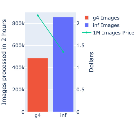
The following charts show a 2-hour run in which Inf1 provides higher throughout and lower latency. The Inf1 instances achieved up to 1.85 times higher throughput and 37% lower cost per image when compared to the most optimized Amazon EC2 G4 GPU-based instances.

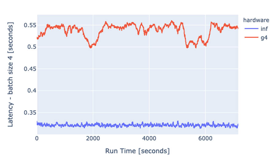
In addition, the following graph records the P90 inference latency is 60% lower on Inf1, and with significant lower variance compared to the G4 instances.

When you use the AWS Neuron data type auto-casting feature, there is no measurable degradation in accuracy. The compiler automatically converts the pipeline to mixed precision with BF16 data types for increased performance. The model reaches 48.7% mean average precision—thanks to the state-of-the-art YOLOv4 model implementation.

About AWS Inferentia and AWS Neuron SDK

AWS Inferentia chips are custom built by AWS to provide high-inference performance, with the lowest cost of inference in the cloud, with seamless features such as auto-conversion of trained FP32 models to Bfloat16, and elasticity in its machine learning (ML) models’ compute architecture, which supports a wide range of model types from image recognition, object detection, natural language processing (NLP), and modern recommender models.

AWS Neuron is a software development kit (SDK) consisting of a compiler, runtime, and profiling tools that optimize the ML inference performance of the Inferentia chips. Neuron is natively integrated with popular ML frameworks such as TensorFlow and PyTorch, and comes pre-installed in the AWS Deep Learning AMIs. Therefore, deploying deep learning models on AWS Inferentia is done in the same familiar environment used in other platforms, and your applications benefit from the boost in performance and lowest cost.

Since its launch, the Neuron SDK has seen dramatic improvement in the breadth of models that deliver high performance at a fraction of the cost. This includes NLP models like the popular BERT, image classification models (ResNet, VGG), and object detection models (OpenPose and SSD). The latest Neuron release (1.8.0) provides optimizations that improve performance of YOLO v3 and v4, VGG16, SSD300, and BERT. It also improves operational deployments of large-scale inference applications, with a session management agent incorporated into all supported ML frameworks and a new Neuron tool that allows you to easily scale monitoring of large fleets of Inference applications.

You Only Look Once

Object detection stands out as a computer vision (CV) task that has seen large accuracy improvements (average precision at 50 IoU > 70) due to deep learning model architectures. An object detection model tries to localize and classify objects in an image, allowing for applications ranging from real-time inspection of manufacturing defects to medical imaging and tracking your favorite player and ball on a soccer match.

Addressing the real-time inference challenges of such computer vision tasks is key for deploying these models at scale.

YOLO is part of the deep learning (DL) single-stage object detection model family, which includes models such as Single-Shot Detector (SSD) and RetinaNet. These models are usually built from stacking a backbone, neck, and head neural network that together perform detection and classification tasks. The main predictions are bounding boxes for identified objects and associated classes.

The backbone network takes care of extracting features of the input image, while the head gets trained on the supervised task, to predict the edges of the bounding box and classify its contents. The addition of a neck neural network allows for the head network to process features from intermediate steps of the backbone. The whole pipeline processes the images only once, hence the name You Only Look Once (YOLO).

On the other hand, models with two-stage detectors process further features from the previous convolutional layers to obtain proposals of regions, prior to generating object class prediction. In this way, the network focuses on detecting and classifying objects on regions of high object probability.

The following diagram illustrates this architecture (from YOLOv4: Optimal Speed and Accuracy of Object Detection, arXiv:2004.10934v1).

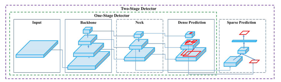
Single-stage models allow for multiple predictions of the same object in a single image. These predictions get disambiguated later by a process called non-max suppression (NMS), which takes care of leaving only the highest probability bounding box and label for the object. It’s a less computationally costly workflow than the two-stage approach.

Models like YOLO are all about performance. Its latest incarnation, version 4, aims at pushing the prediction accuracy further. The research paper YOLOv4: Optimal Speed and Accuracy of Object Detection shows how real-time inference can be achieved above the human perception of around 30 frames per second (FPS). In this post, you explore ways to push the performance of this model even further and use AWS Inferentia as a cost-effective hardware accelerator for real-time object detection.

Prerequisites

For this walkthrough, you need an AWS account with access to the AWS Management Console and the ability to create Amazon Elastic Compute Cloud (Amazon EC2) instances with public-facing IP.

Working knowledge of AWS Deep Learning AMIs and Jupyter notebooks with Conda environments is beneficial, but not required.

Building a YOLOv4 predictor from a pre-trained model

To start building the model, set up an inf1.2xlarge EC2 instance in AWS, with 8 vCPU cores and 16 GB of memory. The Inf1 instance allows for optimizing the ratio between CPU and Inferentia devices through the selection of inf1.xlarge or inf1.2xlarge. We found that for YOLOv4, the optimal CPU to accelerator balance is achieved with inf.2xlarge. Going up to the second size instance improves throughput for a lower cost per image. Use the AWS Deep Learning AMI (Ubuntu 18.04) version 34.0—ami-06a25ee8966373068—in the US East (N. Virginia) Region. This AMI comes pre-packaged with the Neuron SDK and the required Neuron runtime for AWS Inferentia. For more information about running AWS Deep Learning AMIs on EC2 instances, see Launching and Configuring a DLAMI.

Next you can connect to the instance through SSH, activate the aws_neuron_tensorflow_p36 Conda environment, and update the Neuron compiler to the latest release. The compilation script depends on requirements listed in the YOLOv4 tutorial posted on the Neuron GitHub repo. Install them by running the following code in the terminal:

pip install neuron-cc tensorflow-neuron requests pillow matplotlib pycocotools==2.0.1 torch~=1.5.0 --force --extra-index-url=https://pip.repos.neuron.amazonaws.com

You can also run the following steps directly from the provided Jupyter notebook. If doing so, skip to the Running a performance benchmark on Inferentia section to explore the performance benefits of running YOLOv4 on AWS Inferentia.

The benchmark of the models requires an object detection validation dataset. Start by downloading the COCO 2017 validation dataset. The COCO (Common Objects in Context) is a large-scale object detection, segmentation, and captioning dataset, with over 300,000 images and 1.5 million object instances. The 2017 version of COCO contains 5,000 images for validation.

To download the dataset, enter the following code on the terminal:

curl -LO http://images.cocodataset.org/zips/val2017.zip
curl -LO http://images.cocodataset.org/annotations/annotations_trainval2017.zip
unzip -q val2017.zip
unzip annotations_trainval2017.zip

When the download is complete, you should see a val2017 and an annotations folder available in your working directory. At this stage, you’re ready to build and compile the model.

The GitHub repo contains the script yolo_v4_coco_saved_model.py for downloading the pretrained weights of a PyTorch implementation of YOLOv4, and the model definition for YOLOv4 using TensorFlow 1.15 and Keras. The code was adapted from an earlier implementation and converts the PyTorch checkpoint to a Keras h5 saved model. This implementation of YOLOv4 is optimized to run on AWS Inferentia. For more information about optimizations, see Working with YOLO v4 using AWS Neuron SDK.

To download, convert, and save your Keras model to the yolo_v4_coco_saved_model folder, enter the following code:

python3 yolo_v4_coco_saved_model.py ./yolo_v4_coco_saved_model

To instantiate a new predictor from the saved model, use tf.contrib.predictor.from_saved_model('./yolo_v4_coco_saved_model') on your inference script.

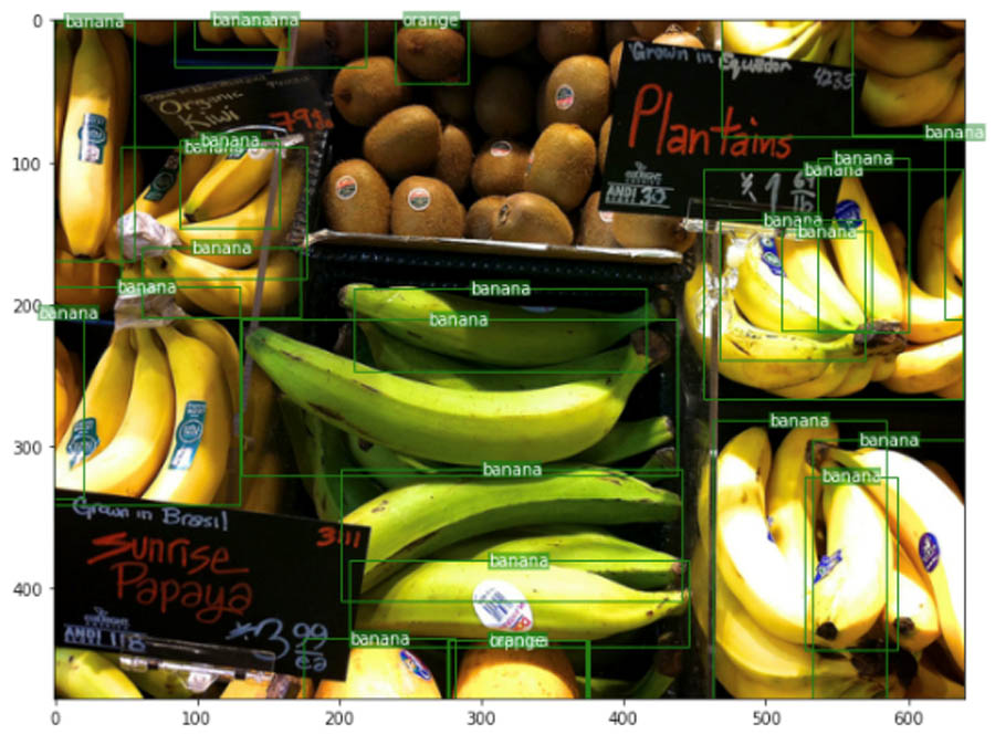
The following code implements a single batch predictor and image annotation script, so you can test the saved model:

import json
import tensorflow as tf
from PIL import Image
import matplotlib.pyplot as plt
import matplotlib.patches as patches

yolo_pred_cpu = tf.contrib.predictor.from_saved_model('./yolo_v4_coco_saved_model')
image_path = './val2017/000000581781.jpg'
with open(image_path, 'rb') as f:
    feeds = {'image': [f.read()]}

results = yolo_pred_cpu(feeds)

# load annotations to decode classification result
with open('./annotations/instances_val2017.json') as f:
    annotate_json = json.load(f)
label_info = {idx+1: cat['name'] for idx, cat in enumerate(annotate_json['categories'])}

# draw picture and bounding boxes
fig, ax = plt.subplots(figsize=(10, 10))
ax.imshow(Image.open(image_path).convert('RGB'))

wanted = results['scores'][0] > 0.1

for xyxy, label_no_bg in zip(results['boxes'][0][wanted], results['classes'][0][wanted]):
    xywh = xyxy[0], xyxy[1], xyxy[2] - xyxy[0], xyxy[3] - xyxy[1]
    rect = patches.Rectangle((xywh[0], xywh[1]), xywh[2], xywh[3], linewidth=1, edgecolor='g', facecolor='none')
    ax.add_patch(rect)
    rx, ry = rect.get_xy()
    rx = rx + rect.get_width() / 2.0
    ax.annotate(label_info[label_no_bg + 1], (rx, ry), color='w', backgroundcolor='g', fontsize=10,
                ha='center', va='center', bbox=dict(boxstyle='square,pad=0.01', fc='g', ec='none', alpha=0.5))
plt.show()

The performance in this setup isn’t optimal because you ran YOLO only on CPU. Despite the native parallelization from TensorFlow, the eight cores aren’t enough to bring the inference time close to real time. For that, you use AWS Inferentia.

Compiling YOLOv4 to run on AWS Inferentia

The compilation of YOLOv4 uses the TensorFlow-Neuron API tfn.saved_mode.compile, working directly with the saved model directory created before. To further reduce the Neuron runtime overhead, two extra arguments are added to the compiler call: no_fuse_ops and minimum_segment_size.

The first argument, no_fuse_ops, partitions the graph prior to casting the FP16 tensors running in the sub-graph back to FP32, as defined in the model script. This allows for operations that run more efficiently on CPU to be skipped while the Neuron compiler runs its automatic smart partitioning. The argument minimum_segment_size sets the minimum number of operations in a sub-graph, to enforce trivial compilable sections to run on CPU. For more information, see Reference: TensorFlow-Neuron Compilation API.

To compile the model, enter the following code:

import shutil
import tensorflow as tf
import tensorflow.neuron as tfn


def no_fuse_condition(op):
    return any(op.name.startswith(pat) for pat in ['reshape', 'lambda_1/Cast', 'lambda_2/Cast', 'lambda_3/Cast'])

with tf.Session(graph=tf.Graph()) as sess:
    tf.saved_model.loader.load(sess, ['serve'], './yolo_v4_coco_saved_model')
    no_fuse_ops = [op.name for op in sess.graph.get_operations() if no_fuse_condition(op)]

shutil.rmtree('./yolo_v4_coco_saved_model_neuron', ignore_errors=True)

result = tfn.saved_model.compile(
                './yolo_v4_coco_saved_model', './yolo_v4_coco_saved_model_neuron',
                # we partition the graph before casting from float16 to float32, to help reduce the output tensor size by 1/2
                no_fuse_ops=no_fuse_ops,
                # to enforce trivial compilable subgraphs to run on CPU
                minimum_segment_size=100,
                batch_size=1,
                dynamic_batch_size=True,
)

print(result)

On an inf1.2xlarge, the compilation takes only a few minutes and outputs the ratio of the graph operations run on the AWS Inferentia chip. For our model, it’s approximately 79%. As mentioned earlier, to optimize the compiled model for performance, the target of the compilation shouldn’t be to maximize operations on the AWS inferential chip, but to balance the use of the available CPUs for efficient combined hardware utilization.

AWS Inferentia is designed to reach peak throughput at small—usually single-digit—batch sizes. When optimizing a specific model for throughput, explore compiling the model with different values of the batch_size argument and test what batch size yields the maximum throughput for your model. In the case of our YOLOv4 model, the best batch size is 1.

Replace the model path on the predictor instantiation to tf.contrib.predictor.from_saved_model('./yolo_v4_coco_saved_model_neuron') for a comparison with the previous CPU only inference. You get similar detection accuracy at a fraction of the inference time, approximately 40 milliseconds.

Setting up a benchmarking pipeline

To set up a performance measuring pipeline, create a multi-threaded loop running inference on all the COCO images downloaded. The code available in the notebook adapts the original implementation of the eval function. The following adapted version implements a ThreadPoolExecutor to send four parallel prediction calls at a time:

from concurrent import futures

def evaluate(yolo_predictor, images, eval_pre_path, anno_file, eval_batch_size, _clsid2catid):
    batch_im_id_list, batch_im_name_list, batch_img_bytes_list = get_image_as_bytes(images, eval_pre_path)

    # warm up
    yolo_predictor({'image': np.array(batch_img_bytes_list[0], dtype=object)})

    with futures.ThreadPoolExecutor(4) as exe:
        fut_im_list = []
        fut_list = []
        start_time = time.time()
        for batch_im_id, batch_im_name, batch_img_bytes in zip(batch_im_id_list, batch_im_name_list, batch_img_bytes_list):
            if len(batch_img_bytes) != eval_batch_size:
                continue
            fut = exe.submit(yolo_predictor, {'image': np.array(batch_img_bytes, dtype=object)})
            fut_im_list.append((batch_im_id, batch_im_name))
            fut_list.append(fut)
        bbox_list = []
        count = 0
        for (batch_im_id, batch_im_name), fut in zip(fut_im_list, fut_list):
            results = fut.result()
            bbox_list.extend(analyze_bbox(results, batch_im_id, _clsid2catid))
            for _ in batch_im_id:
                count += 1
                if count % 100 == 0:
                    print('Test iter {}'.format(count))
        
        print('==================== Performance Measurement ====================')
        print('Finished inference on {} images in {} seconds'.format(len(images), time.time() - start_time))
        print('=================================================================')
    
    # start evaluation
    box_ap_stats = bbox_eval(anno_file, bbox_list)
    return box_ap_stats

Additional helper functions are used to calculate average precision scores of the deployed model.

Running a performance benchmark on Inferentia

To run the COCO evaluation and benchmark the time to infer over the 5,000 images, run the evaluate function as shown in the following code:

val_coco_root = './val2017'
val_annotate = './annotations/instances_val2017.json'
clsid2catid = {0: 1, 1: 2, 2: 3, 3: 4, 4: 5, 5: 6, 6: 7, 7: 8, 8: 9, 9: 10, 10: 11, 11: 13, 12: 14, 13: 15, 14: 16,
               15: 17, 16: 18, 17: 19, 18: 20, 19: 21, 20: 22, 21: 23, 22: 24, 23: 25, 24: 27, 25: 28, 26: 31,
               27: 32, 28: 33, 29: 34, 30: 35, 31: 36, 32: 37, 33: 38, 34: 39, 35: 40, 36: 41, 37: 42, 38: 43,
               39: 44, 40: 46, 41: 47, 42: 48, 43: 49, 44: 50, 45: 51, 46: 52, 47: 53, 48: 54, 49: 55, 50: 56,
               51: 57, 52: 58, 53: 59, 54: 60, 55: 61, 56: 62, 57: 63, 58: 64, 59: 65, 60: 67, 61: 70, 62: 72,
               63: 73, 64: 74, 65: 75, 66: 76, 67: 77, 68: 78, 69: 79, 70: 80, 71: 81, 72: 82, 73: 84, 74: 85,
               75: 86, 76: 87, 77: 88, 78: 89, 79: 90}
eval_batch_size = 8

with open(val_annotate, 'r', encoding='utf-8') as f2:
    for line in f2:
        line = line.strip()
        dataset = json.loads(line)
        images = dataset['images']

box_ap = evaluate(yolo_pred, images, val_coco_root, val_annotate, eval_batch_size, clsid2catid)

When the evaluation is complete, you see logs on the screen like the following:

…

Test iter 4500
Test iter 4600
Test iter 4700
Test iter 4800
Test iter 4900
==================== Performance Measurement ====================
Finished inference on 5000 images in 47.50522780418396 seconds
=================================================================

…

Accumulating evaluation results...
DONE (t=6.78s).
 Average Precision  (AP) @[ IoU=0.50:0.95 | area=   all | maxDets=100 ] = 0.487
 Average Precision  (AP) @[ IoU=0.50      | area=   all | maxDets=100 ] = 0.741
 Average Precision  (AP) @[ IoU=0.75      | area=   all | maxDets=100 ] = 0.531
 Average Precision  (AP) @[ IoU=0.50:0.95 | area= small | maxDets=100 ] = 0.330
 Average Precision  (AP) @[ IoU=0.50:0.95 | area=medium | maxDets=100 ] = 0.546
 Average Precision  (AP) @[ IoU=0.50:0.95 | area= large | maxDets=100 ] = 0.604
 Average Recall     (AR) @[ IoU=0.50:0.95 | area=   all | maxDets=  1 ] = 0.357
 Average Recall     (AR) @[ IoU=0.50:0.95 | area=   all | maxDets= 10 ] = 0.573
 Average Recall     (AR) @[ IoU=0.50:0.95 | area=   all | maxDets=100 ] = 0.601
 Average Recall     (AR) @[ IoU=0.50:0.95 | area= small | maxDets=100 ] = 0.430
 Average Recall     (AR) @[ IoU=0.50:0.95 | area=medium | maxDets=100 ] = 0.657
 Average Recall     (AR) @[ IoU=0.50:0.95 | area= large | maxDets=100 ] = 0.744

At 5,000 images processed in 47 seconds, this deployment achieves 106 FPS, 3.5 times faster than the real-time threshold of 30 FPS. The research paper YOLOv4: Optimal Speed and Accuracy of Object Detection lists the results for batch one performance over the same COCO 2017 dataset running on a NVIDIA Volta GPU, such as the V100. The largest frame rate obtained was 96 FPS, at 41.2% mAP. Our model architecture and deployment achieves higher mAP, 48.7%, with a higher frame rate.

To have a direct comparison between AWS Inferentia, NVIDIA Volta, and Turing architectures, we replicated the same experiment in two GPU based instances, g4dn.xlarge and p3.2xlarge, by running the exact same model prior to compilation, with no further GPU optimization. This time we achieved 39 FPS and 111 FPS for the g4dn.xlarge and p3.2xlarge, respectively.

A YOLO model deployed in production usually doesn’t see a defined batch of 5,000 images at a time. To measure production like performance, we set up a prediction-only multi-threaded pipeline that runs inference for extended periods.

For a total time of 2 hours, we continually ran 8 parallel prediction calls with a batch of 4 images on each, totaling 32 images at a time. To maximize GPU throughput and try to decrease the performance gap between the Inf1 and G4 instances, we use the TensorFlow XLA compiler. This setup mimics a live endpoint behavior running at maximum throughput.

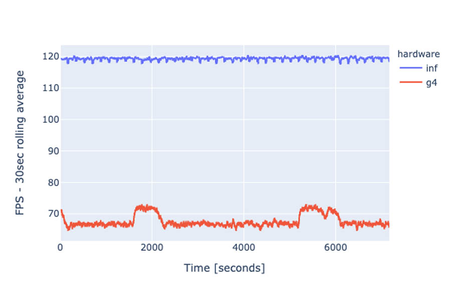
GPU thermal throttling

In contrast to AWS Inferentia chips, GPU throughput is inversely proportional to GPU temperature. GPU temperature can vary on endpoints running for extended periods at high throughput, which leads to FPS and latency fluctuations. This effect is known as thermal throttling. Some production systems can define a limit throughput below the maximum achievable to avoid performance swings over time. The following graph shows the average FPS over 30 second increments for the duration of the test . We observed up to 12% variation of the FPS rolling average on the GPU instance. On AWS Inferentia, this variation is below 3% for a substantially larger FPS average.

During the 2-hour period, we ran inference on over 856,000 images on the inf1.2xlarge instance. On the g4dn.xlarge, the maximum number of inferences achieved was 486,000. That amounts to 76% more images processed over the same amount of time using AWS Inferentia! Latency averages for batch 4 inference are also 60% lower for AWS Inferentia.

Using the total throughput collected during our 2-hour test, we calculated that the price of running 1 million inferences is $1.362 on an inf1.xlarge in the us-east-1 Region. For the g4dn.xlarge, the price is $2.163—a 37% price reduction for the YOLOv4 object detection pipeline on AWS Inferentia.

Safely shutting down and cleaning up

On the Amazon EC2 console, choose the instances used to perform the benchmark, and choose Terminate from the Actions drop-down menu. Stopping the instance discards data stored only in the instance’s home volume. You can persist the compiled model in an Amazon Simple Storage Service (S3) bucket, so it can be reused later. If you’ve made changes to the code inside the instances, remember to persist those as well.

Conclusion

In this post, you walked through the steps of optimizing a TensorFlow YOLOv4 model to run on AWS Inferentia. You explored AWS Neuron optimizations that yield better model performance with improved average precision, and in a much more cost-effective way. In production, the Neuron compiled model is up to 37% less expensive in the long run, with little throughput and latency fluctuations, when compared to the most optimized GPU instance.

Some of the steps described in this post also apply to other ML model types and frameworks. For more information, see the AWS Neuron SDK GitHub repo.

Learn more about the AWS Inferentia chip and the Amazon EC2 Inf1 instances to get started with running your own custom ML pipelines on AWS Inferentia using the Neuron SDK.

About the Authors

Fabio Nonato de Paula is a Principal Solutions Architect for Autonomous Computing in AWS. He works with large-scale deployments of ML and AI for autonomous and intelligent systems. Fabio is passionate about democratizing access to accelerated computing and distributed ML. Outside of work, you can find Fabio riding his motorcycle on the hills of Livermore valley or reading ComiXology.

Haichen Li is a software development engineer in the AWS Neuron SDK team. He works on integrating machine learning frameworks with the AWS Neuron compiler and runtime systems, as well as developing deep learning models that benefit particularly from the Inferentia hardware.

Samuel Jacob is a senior software engineer in the AWS Neuron team. He works on AWS Neuron runtime to enable high performance inference data paths between AWS Neuron SDK and AWS Inferentia hardware. He also works on tools to analyze and improve AWS Neuron SDK performance. Outside of work, you can catch him playing video games or tinkering with small boards such as RaspberryPi.