Churn prediction using multimodality of text and tabular features with Amazon SageMaker Jumpstart

Amazon SageMaker JumpStart is the Machine Learning (ML) hub of SageMaker providing pre-trained, publicly available models for a wide range of problem types to help you get started with machine learning.

Understanding customer behavior is top of mind for every business today. Gaining insights into why and how customers buy can help grow revenue. Customer churn is a problem faced by a wide range of companies, from telecommunications to banking, where customers are typically lost to competitors. It’s in a company’s best interest to retain existing customers instead of acquiring new customers, because it usually costs significantly more to attract new customers. When trying to retain customers, companies often focus their efforts on customers who are more likely to leave. User behavior and customer support chat logs can contain valuable indicators on the likelihood of a customer ending the service. In this solution, we train and deploy a churn prediction model that uses a state-of-the-art natural language processing (NLP) model to find useful signals in text. In addition to textual inputs, this model uses traditional structured data inputs such as numerical and categorical fields.

Multimodality is a multi-disciplinary research field that addresses some of the original goals of artificial intelligence by integrating and modeling multiple modalities. This post aims to build a model that can process and relate information from multiple modalities such as tabular and textual features.

We show you how to train, deploy and use a churn prediction model that has processed numerical, categorical, and textual features to make its prediction. Although we dive deep into a churn prediction use case in this post, you can use this solution as a template to generalize fine-tuning pre-trained models with your own dataset, and subsequently run hyperparameter optimization (HPO) to improve accuracy. You can even replace the example dataset with your own and run it end to end to solve your own use cases. The solution outlined in the post is available on GitHub.

JumpStart solution templates

Amazon SageMaker JumpStart provides one-click, end-to-end solutions for many common ML use cases. Explore the following use cases for more information on available solution templates:

• Demand forecasting
• Credit rating prediction
• Fraud detection
• Computer vision
• Extract and analyze data from documents
• Predictive maintenance
• Churn prediction
• Personalized recommendations
• Reinforcement learning
• Healthcare and life sciences
• Financial pricing

The JumpStart solution templates cover a variety of use cases, under each of which several different solution templates are offered (this Document Understanding solution is under the “Extract and analyze data from documents” use case).

Choose the solution template that best fits your use case from the JumpStart landing page. For more information on specific solutions under each use case and how to launch a JumpStart solution, see Solution Templates.

Solution overview

The following figure demonstrates how you can use this solution with Amazon SageMaker components. The SageMaker training jobs are used to train the various NLP models, and SageMaker endpoints are used to deploy the models in each stage. We use Amazon Simple Storage Service (Amazon S3) alongside SageMaker to store the training data and model artifacts, and Amazon CloudWatch to log training and endpoint outputs.

We approach solving the churn prediction problem with the following steps:

1. Data exploration to prepare the data to be ML ready.
2. Train a multimodal model with a Hugging Face sentence transformer and Scikit-learn random forest classifier.
3. Further improve the model performance with HPO using SageMaker automatic model tuning.
4. Train two AutoGluon multimodal models: an AutoGluon multimodal weighted/stacked ensemble model, and an AutoGluon multimodal fusion model.
5. Evaluate and compare the model performances on the holdout test data.

Prerequisites

To try out the solution in your own account, make sure that you have the following in place:

• An AWS account. If you don’t have an account, you can sign up for one.
• The solution outlined in the post is part of SageMaker JumpStart. To run this JumpStart solution and have the infrastructure deploy to your AWS account, you must create an active Amazon SageMaker Studio instance (see Onboard to Amazon SageMaker Studio). When your Studio instance is ready, use the instructions in JumpStart to launch the solution.
• When running this notebook on Studio, you should make sure the Python 3 (PyTorch 1.10 Python 3.8 CPU Optimized) image/kernel is used.

You can install the required packages as outlined in the solution to run this notebook:

• Scikit-learn
• Sentence transformer
• Hugging Face Transformers
• AutoGluon

Open the churn prediction use case

On the Studio console, choose Solutions, models, example notebooks under Quick start solutions in the navigation pane. Navigate to the Churn Prediction with Text solution in JumpStart.

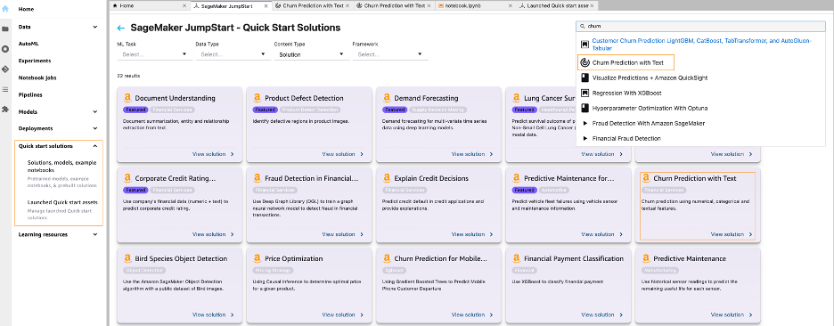
Now we can take a closer look at some of the assets that are included in this solution.

Data exploration

First let’s download the test, validate, and train dataset from the source S3 bucket and upload it to our S3 bucket. The following screenshot shows us 10 observations of the training data.

Let’s begin exploring the train and validation dataset.

As you can see, we have different features such as CustServ Calls, Day Charge, and Day Calls that we use to predict the target column y (whether the customer left the service).

y is known as the target attribute: the attribute that we want the ML model to predict. Because the target attribute is binary, our model performs binary prediction, also known as binary classification.

There are 21 features, including the target variable. The number of examples for training and validation data are 43,000 and 5,000, respectively.

The following screenshot shows the summary statistics of the training dataset.

We have explored the dataset and split it into training, validation, and test sets. The training and validation set is used for training and HPO. The test set is used as the holdout set for model performance evaluation. We now carry out feature engineering steps and then fit the model.

Fit a multimodal model with a Hugging Face sentence transformer and Scikit-learn random forest classifier

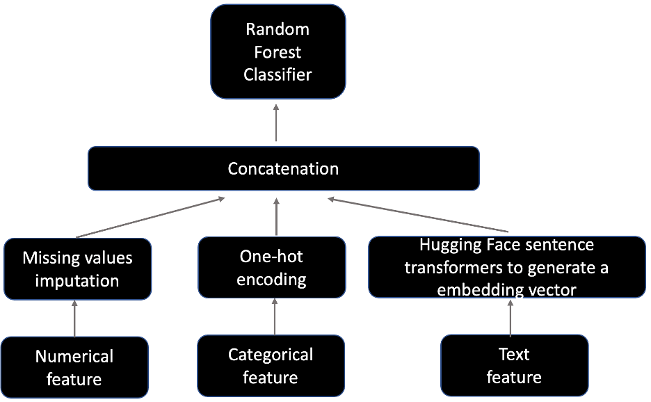
The model training consists of two components: a feature engineering step that processes numerical, categorical, and text features, and a model fitting step that fits the transformed features into a Scikit-learn random forest classifier.

For the feature engineering, we complete the following steps:

1. Fill in the missing values for numerical features.
2. Encode categorical features into one-hot values, where the missing values are counted as one of the categories for each feature.
3. Use a Hugging Face sentence transformer to encode the text feature to generate a X-dimensional dense vector, where the value of X depends on a particular sentence transformer.

We choose the top three most downloaded sentence transformer models and use them in the following model fitting and HPO. Specifically, we use all-MiniLM-L6-v2, multi-qa-mpnet-base-dot-v1, and paraphrase-MiniLM-L6-v2. For hyperparameters of the random forest classifier, refer to the GitHub repo.

The following figure depicts the model architecture diagram.

There are many hyperparameters you can tune, such as n-estimators, max-depth, and bootstrap. For more details, refer to the GitHub repo.

For demonstration purposes, we only use numerical features CustServ Calls and Account Length, categorical features plan, and limit, and text feature text to fit the model. Multiple features should be separated by ,.

hyperparameters = {
    "n-estimators": 50,
    "min-impurity-decrease": 0.0,
    "ccp-alpha": 0.0,   
    "sentence-transformer": "sentence-transformers/all-MiniLM-L6-v2",
    "criterion": "gini",
    "max-depth": 6,
    "boostrap": "True",
    "min-samples-split": 4,
    "min-samples-leaf": 1,
    "balanced-data": True,
    "numerical-feature-names": "CustServ Calls,Account Length",
    "categorical-feature-names": "plan,limit",
    "textual-feature-names": "text",
    "label-name": "y"
}

current_folder = utils.get_current_folder(globals())
estimator = PyTorch(
    framework_version='1.5.0',
    py_version='py3',
    entry_point='entry_point.py',
    source_dir=str(Path(current_folder, '../containers/huggingface_transformer_randomforest').resolve()),
    hyperparameters=hyperparameters,
    role=config.IAM_ROLE,
    instance_count=1,
    instance_type=config.TRAINING_INSTANCE_TYPE,
    output_path='s3://' + str(Path(config.S3_BUCKET, config.OUTPUTS_S3_PREFIX_RF)),
    code_location='s3://' + str(Path(config.S3_BUCKET, config.OUTPUTS_S3_PREFIX_RF)),
    base_job_name=config.SOLUTION_PREFIX,
    tags=[{'Key': config.TAG_KEY, 'Value': config.SOLUTION_PREFIX}],
    sagemaker_session=sagemaker_session,
    volume_size=30
)

estimator.fit({
    'train': 's3://' + str(Path(config.S3_BUCKET, config.DATASETS_S3_PREFIX, 'train.jsonl')),
    'validation': 's3://' + str(Path(config.S3_BUCKET, config.DATASETS_S3_PREFIX, 'validation.jsonl'))
})

We deploy the model after training is complete:

from sagemaker.serializers import JSONSerializer
from sagemaker.deserializers import JSONDeserializer

predictor = estimator.deploy(
    endpoint_name=endpoint_name,
    instance_type=config.HOSTING_INSTANCE_TYPE,
    initial_instance_count=1,
    serializer=JSONSerializer(),
    deserializer=JSONDeserializer()
)

When calling our new endpoint from the notebook, we use a SageMaker SDK Predictor. A Predictor is used to send data to an endpoint (as part of a request) and interpret the response. JSON is used as the format for both input data and output response because it’s a standard endpoint format and the endpoint response can contain nested data structures.

With our model successfully deployed and our predictor configured, we can try out the churn prediction model on an example input:

data = {
    "CustServ Calls": -20.0,
    "Account Length": 133.12,
    "plan": "D",
    "limit": "unlimited",
    "text": "Well, I've been dealing with TelCom for three months now, and I feel like they're very helpful and responsive to my issues, but for a month now, I've only had one technical support call and that was very long and involved. My phone number was wrong on both contracts, and they gave me a chance to work with TelCom customer service and it was extremely helpful, so I've decided to stick with it. But I would like to have more help in terms of technical support, I haven't had the kind of help with my phone line and I don't have the type of tech support I want. So I would like to negotiate a phone contract, maybe an upgrade from a Sprint plan, or maybe from a Verizon plan.\\nTelCom Agent: Very good."
}
response = predictor.predict(data=[data])

The following code shows the response (probability of churn) from querying the endpoint:

20.09% probability of churn

Note that the probability returned by this model has not been calibrated. When the model gives a probability of churn of 20%, for example, this doesn’t necessarily mean that 20% of customers with a probability of 20% resulted in churn. Calibration is a useful property in certain circumstances, but isn’t required in cases where discrimination between cases of churn and non-churn is sufficient. CalibratedClassifierCV from Scikit-learn can be used to calibrate a model.

Now we query the endpoint using the hold-out test data, which consists of 1,939 examples. The following table summarizes the evaluation results for our multimodal model with a Hugging Face sentence transformer and Scikit-learn random forest classifier.

Model performance is dependent on hyperparameter configurations. Training a model with one set of hyperparameter configurations will not guarantee an optimal model. As a result, we run the HPO process in the following section to further improve model performance.

Fit a multimodal model with HPO

In this section, we further improve the model performance by adding HPO tuning with SageMaker automatic model tuning. SageMaker automatic model tuning, also known as hyperparameter tuning, finds the best version of a model by running many training jobs on your dataset using the algorithm and ranges of hyperparameters that you specify. It then chooses the hyperparameter values that result in a model that performs the best, as measured by a metric that you choose. The best model and its corresponding hyperparameters are selected on the validation data. Next, the best model is evaluated on the hold-out test data, which is the same test data we created in the previous section. Finally, we show that the performance of the model trained with HPO is significantly better than the one trained without HPO.

The following are static hyperparameters we don’t tune and dynamic hyperparameters we want to tune and their searching ranges:

from sagemaker.tuner import ContinuousParameter, IntegerParameter, CategoricalParameter, HyperparameterTuner
hyperparameters = {
    "min_impurity_decrease": 0.0,
    "ccp_alpha": 0.0,
    "numerical-feature-names": "CustServ Calls,Account Length",
    "categorical-feature-names": "plan,limit",
    "textual-feature-names": "text",
    "label-name": "y"
}
hyperparameter_ranges = {
    "sentence-transformer": CategoricalParameter([
    "sentence-transformers/all-MiniLM-L6-v2", "sentence-transformers/multi-qa-mpnet-base-dot-v1", "sentence-transformers/paraphrase-MiniLM-L6-v2"]
    ),
    "criterion": CategoricalParameter(["gini", "entropy"]),
    "max-depth": CategoricalParameter([10, 20, 30, 40, 50, 60, 70, 80, 90, 100, -1]),
    "boostrap": CategoricalParameter(["True", "False"]),
    "min-samples-split": IntegerParameter(2, 10),
    "min-samples-leaf": IntegerParameter(1, 5),
    "n-estimators": CategoricalParameter([100, 200, 400, 800, 1000]),
}

tuning_job_name = f"{config.SOLUTION_PREFIX}-hpo"

current_folder = utils.get_current_folder(globals())
estimator = PyTorch(
    framework_version='1.5.0',
    py_version='py3',
    entry_point='entry_point.py',
    source_dir=str(Path(current_folder, '../containers/huggingface_transformer_randomforest').resolve()),
    hyperparameters=hyperparameters,
    role=config.IAM_ROLE,
    instance_count=1,
    instance_type=config.TRAINING_INSTANCE_TYPE,
    output_path='s3://' + str(Path(config.S3_BUCKET, config.OUTPUTS_S3_PREFIX_RF)),
    code_location='s3://' + str(Path(config.S3_BUCKET, config.OUTPUTS_S3_PREFIX_RF)),
    tags=[{'Key': config.TAG_KEY, 'Value': config.SOLUTION_PREFIX}],
    sagemaker_session=sagemaker_session,
    volume_size=30
)

We define the objective metric name, metric definition (with regex pattern), and objective type for the tuning job.

First, we set the objective as the accuracy score on the validation data (roc auc score on validation data) and defined metrics for the tuning job by specifying the objective metric name and a regular expression (regex). The regular expression is used to match the algorithm’s log output and capture the numeric values of metrics.

objective_metric_name = "roc auc"
metric_definitions = [{"Name": "roc auc", "Regex": "roc auc score on validation data: ([0-9\\.]+)"}]
objective_type = "Maximize"

Next, we specify hyperparameter ranges to select the best hyperparameter values from. We set the total number of tuning jobs as 10 and distribute these jobs on five different Amazon Elastic Compute Cloud (Amazon EC2) instances for running parallel tuning jobs.

Finally, we pass those values to instantiate a SageMaker Estimator object, similar to what we did in the previous training step. Instead of calling the fit function of the Estimator object, we pass the Estimator object in as a parameter to the HyperparameterTuner constructor and call the fit function of it to launch tuning jobs:

tuner = HyperparameterTuner(
    estimator,
    objective_metric_name,
    hyperparameter_ranges,
    metric_definitions,
    max_jobs=18, # increase the maximum number of jobs will likely get better performance
    max_parallel_jobs=3,
    objective_type=objective_type,
    base_tuning_job_name=tuning_job_name,
)

# Launch a SageMaker Tuning job to search for the best hyperparameters
tuner.fit(
    {'train': 's3://' + str(Path(config.S3_BUCKET, config.DATASETS_S3_PREFIX, 'train.jsonl')), 'validation': 's3://' + str(Path(config.S3_BUCKET, config.DATASETS_S3_PREFIX, 'validation.jsonl'))},
    logs=True
)

When the tuning job is complete, we can generate the summary table of all the tuning jobs.

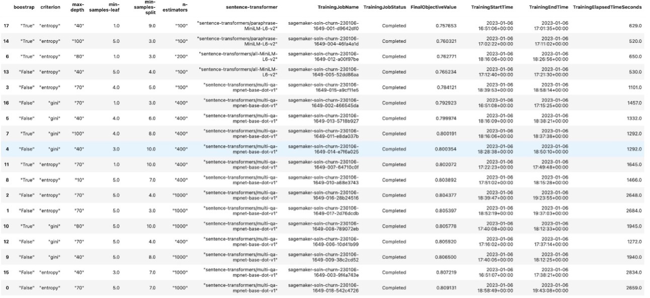
After the tuning jobs are complete, we deploy the model that gives the best evaluation metric score on the validation dataset, perform inference on the same hold-out test dataset we did in the previous section, and compute evaluation metrics.

We can see running HPO with SageMaker automatic model tuning significantly improves the model performance.

In addition to HPO, model performance is also dependent on the algorithm. It’s important to train multiple state-of-the-art algorithms, compare their performance on the same hold-out test data, and pick up the optimal one. Therefore, we train two more AutoGluon multimodal models in the following sections.

Fit an AutoGluon multimodal weighted/stacked ensemble model

There are two types of AutoGluon multimodality:

• Train multiple tabular models as well as the TextPredictor model (utilizing the TextPredictor model inside of TabularPredictor), and then combine them via either a weighted ensemble or stacked ensemble, as explained in AutoGluon-Tabular: Robust and Accurate AutoML for Structured Data
• Fuse multiple neural network models directly and handle raw text (which are also capable of handling additional numerical and categorical columns)

We train a multimodal weighted or stacked ensemble model first in this section, and train a fusion neural network model in the next section.

First, we retrieve the AutoGluon training image:

from sagemaker import image_uris
from sagemaker.estimator import Estimator

train_image_uri = image_uris.retrieve(
    "autogluon",
    region=boto3.Session().region_name,
    version='0.5.2',
    py_version='py38',
    image_scope="training",
    instance_type=config.TRAINING_INSTANCE_TYPE,
)

Next, we pass in hyperparameters. Unlike existing AutoML frameworks that primarily focus on the model or hyperparameter selection, AutoGluonTabular succeeds by ensembling multiple models and stacking them in multiple layers. Therefore, HPO is usually not required for AutoGluon ensemble models.

hyperparameters = {
    "numerical-feature-names": "CustServ Calls,Account Length",
    "categorical-feature-names": "plan,limit",
    "textual-feature-names": "text",
    "label-name": "y",
    "problem_type": "classification", # either classification or regression. For classification, we will identify binary or multiclass classification in the training script
    "eval_metric": "roc_auc",
    "presets": "medium_quality",
    "auto_stack": "False",
    "num_bag_folds": 0,
    "num_bag_sets": 1,
    "num_stack_levels": 0,
    "refit_full": "False",
    "set_best_to_refit_full": "False",
    "save_space": "True",
    "verbosity": 2,
    "pretrained-transformer": "google/electra-small-discriminator"
}

Finally, we create a SageMaker Estimator and call estimator.fit() to start a training job:

# Create SageMaker Estimator instance

training_job_name_ag = f"{config.SOLUTION_PREFIX}-ag"

tabular_estimator_ag = Estimator(
    role=config.IAM_ROLE,
    image_uri=train_image_uri,
    entry_point='train.py',
    source_dir=str(Path(current_folder, '../containers/autogluon_multimodal_ensemble').resolve()),
    instance_count=1,
    instance_type=config.TRAINING_INSTANCE_TYPE,
    max_run=360000,
    hyperparameters=hyperparameters,
    base_job_name=training_job_name_ag,
    output_path='s3://' + str(Path(config.S3_BUCKET, config.OUTPUTS_S3_PREFIX_AG_ENSEMBLE)),
    code_location='s3://' + str(Path(config.S3_BUCKET, config.OUTPUTS_S3_PREFIX_AG_ENSEMBLE)),
    tags=[{'Key': config.TAG_KEY, 'Value': config.SOLUTION_PREFIX}],
)

tabular_estimator_ag.fit(
    {
        'train': 's3://' + str(Path(config.S3_BUCKET, config.DATASETS_S3_PREFIX, 'train.jsonl')),
        'validation': 's3://' + str(Path(config.S3_BUCKET, config.DATASETS_S3_PREFIX, 'validation.jsonl'))
    }, logs=False
)

After training is complete, we retrieve the AutoGluon inference image and deploy the model:

# Retrieve the inference docker container uri
inference_image_uri = image_uris.retrieve(
    "autogluon",
    region=boto3.Session().region_name,
    version='0.5.2',
    py_version='py38',
    image_scope="inference",
    instance_type=config.HOSTING_INSTANCE_TYPE,
)

endpoint_name_ag = f"{config.SOLUTION_PREFIX}-ag-endpoint"

predictor_ag = tabular_estimator_ag.deploy(
    initial_instance_count=1,
    instance_type=config.HOSTING_INSTANCE_TYPE,
    entry_point="inference.py",
    image_uri=inference_image_uri,
    source_dir=str(Path(current_folder, '../containers/autogluon_multimodal_ensemble').resolve()),
    endpoint_name=endpoint_name_ag,
)

After we deploy the endpoints, we query the endpoint using the same test set and compute evaluation metrics. In the following table, we can see AutoGluon multimodal ensemble improves about 3% in ROC AUC compared with the BERT sentence transformer and random forest with HPO.

Fit an AutoGluon multimodal fusion model

The following diagram illustrates the architecture of the model. For details, see AutoMM for Text + Tabular – Quick Start.

Internally, we use different networks to encode the text columns, categorical columns, and numerical columns. The features generated by individual networks are aggregated by a late-fusion aggregator. The aggregator can output both the logits or score predictions.

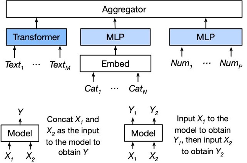
Here, we use the pretrained NLP backbone to extract the text features and then use two other towers to extract the feature from the categorical column and numerical column.

In addition, to deal with multiple text fields, we separate these fields with the [SEP] token and alternate 0s and 1s as the segment IDs, as shown in the following diagram.

Similarly, we follow instructions in the previous section to train and deploy the AutoGluon multimodal fusion model:

# Create SageMaker Estimator instance
training_job_name_ag_fusion = f"{config.SOLUTION_PREFIX}-ag-fusion"

hyperparameters = {
    "numerical-feature-names": "CustServ Calls,Account Length",
    "categorical-feature-names": "plan,limit",
    "textual-feature-names": "text",
    "label-name": "y",
    "problem_type": "classification", # either classification or regression. For classification, we will identify binary or multiclass classification in the training script
    "eval_metric": "roc_auc",
    "verbosity": 2,
    "pretrained-transformer": "google/electra-small-discriminator",
}

tabular_estimator_ag_fusion = Estimator(
    role=config.IAM_ROLE,
    image_uri=train_image_uri,
    entry_point='train.py',
    source_dir=str(Path(current_folder, '../containers/autogluon_multimodal_fusion').resolve()),
    instance_count=1,
    instance_type=config.TRAINING_INSTANCE_TYPE,
    max_run=360000,
    hyperparameters=hyperparameters,
    base_job_name=training_job_name_ag_fusion,
    output_path='s3://' + str(Path(config.S3_BUCKET, config.OUTPUTS_S3_PREFIX_AG_FUSION)),
    code_location='s3://' + str(Path(config.S3_BUCKET, config.OUTPUTS_S3_PREFIX_AG_FUSION)),
    tags=[{'Key': config.TAG_KEY, 'Value': config.SOLUTION_PREFIX}],
)

tabular_estimator_ag_fusion.fit(
    {
        'train': 's3://' + str(Path(config.S3_BUCKET, config.DATASETS_S3_PREFIX, 'train.jsonl')),
        'validation': 's3://' + str(Path(config.S3_BUCKET, config.DATASETS_S3_PREFIX, 'validation.jsonl'))
    }, logs=False
)

The following table summarizes the evaluation results for the AutoGluon multimodal fusion model, along with those of three models that we evaluated in the previous sections. We can see the AutoGluon multimodal ensemble and multimodal fusion models achieve the best performance.

Note that the results and relative performance between these models depend on the dataset you use for training. These results are representative, and even though the tendency for certain algorithms to perform better is based on relevant factors, the balance in performance might change given a different data distribution. You can replace the example dataset with your own data to determine what model works best for you.

Demo notebook

You can use the demo notebook to send example data to already-deployed model endpoints. The demo notebook quickly allows you to get hands-on experience by querying the example data. After you launch the Churn Prediction with Text solution, open the demo notebook by choosing Use Endpoint in Notebook.

Clean up

When you’ve finished with this solution, make sure that you delete all unwanted AWS resources by choosing Delete all resources.

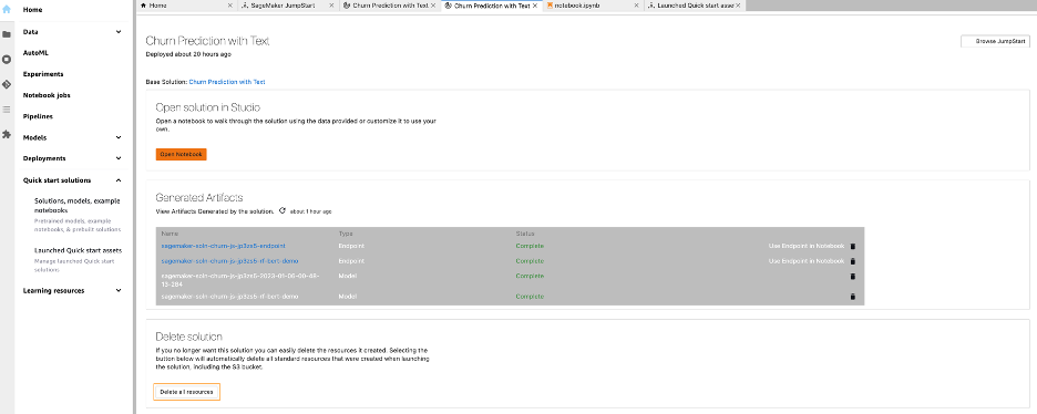
Note that you need to manually delete any additional resources that you may have created in this notebook.

Conclusion

In this post, we showed how you can use Sagemaker JumpStart to predict churn using multimodality of text and tabular features.

If you’re interested in learning more about customer churn models, check out the following posts:

• Analyze customer churn probability using call transcription and customer profiles with Amazon SageMaker
• Preventing customer churn by optimizing incentive programs using stochastic programming
• Build, tune, and deploy an end-to-end churn prediction model using Amazon SageMaker Pipelines

About the Authors

Dr. Xin Huang is an Applied Scientist for Amazon SageMaker JumpStart and Amazon SageMaker built-in algorithms. He focuses on developing scalable machine learning algorithms. His research interests are in the area of natural language processing, explainable deep learning on tabular data, and robust analysis of non-parametric space-time clustering. He has published many papers in ACL, ICDM, KDD conferences, and Royal Statistical Society: Series A journal.

Rajakumar Sampathkumar is a Principal Technical Account Manager at AWS, providing customers guidance on business-technology alignment and supporting the reinvention of their cloud operation models and processes. He is passionate about cloud and machine learning. Raj is also a machine learning specialist and works with AWS customers to design, deploy, and manage their AWS workloads and architectures.