A personalized ‘shop-by-style’ experience using PyTorch on Amazon SageMaker and Amazon Neptune

Remember the screech of the dial-up and plain-text websites? It was in that era that the Amazon.com website launched in the summer of 1995.

Like the rest of the web, Amazon.com has gone through a digital experience makeover that includes slick web controls, rich media, multi-channel support, and intelligent content placement.

Nonetheless, there are certain aspects of the experience that have remained relatively constant. Navigation for an online shopping experience still includes running searches, following recommendations, and textual navigation. However, with the democratization of IoT and AI, this is the moment for innovators to change the status quo.

Amazon, true to its culture of continuous innovation, has been experimenting with creating new customer experiences. Products like Echo Look use machine learning (ML) to allow a customer to ask “Alexa, how do I look?” Then Alexa gives you real-time feedback on your outfit, and you receive smart, specific, and fun styling advice.

In this blog post, I’ll show you how easy it is to create a shop-by-style experience. I’ll introduce you to AWS services that can put you on the right path for rapid experimentation and innovation of new customer experiences.

To demonstrate the shop-by-style experience, we’re going to use the product catalog from Zappos.com. The catalog consists of a variety of footwear from a large selection of brands that include shoes, boots, and sandals of various types.

Footwear is a great example of where a shop-by-style experience could be helpful. If you’re like me, you don’t know exactly what you’re looking for when you walk into a shoe store. Maybe you have some general preferences like color or a brand’s signature style, so you gravitate to specific selections on the shoe rack.

We can replicate this experience in the digital world with the help of machine learning. I’ll show you how you can deliver a quality experience quickly and economically with the help of the AWS Cloud.

The following animated GIF illustrates the concept. The large image displays the shopper’s current selection, and an ML model is used to identify six products from the catalog that are the most stylistically similar to the selection.

You can implement creative variations of this experience. For instance, your app could share products visually similar to those that the user’s favorite celebrity wears, or your app could use stylistic similarity as one of the features that influence product recommendations.

Solution architecture

Our minimalist solution architecture leverages the following AWS services:

Our solution makes use of Amazon SageMaker to manage the end-to-end process of building a deep learning (DL) model. We’ll use PyTorch, which is a DL framework favored by many for rapid prototyping. Together, PyTorch and Amazon SageMaker enable rapid development of a custom model tailored to our needs. However, depending on your preferences, Amazon SageMaker provides you with the choice of using other frameworks like TensorFlow, Keras, and Gluon.

Next, we’ll generate similarity scores using our model, store this data in our Amazon data lake, and use AWS Glue to catalog and transform the data so that it can be loaded into Amazon Neptune, a managed graph database.

Amazon Neptune provides us with a way to build graphical visualizations to analyze the similarity between our products. It’s also designed to serve as an operational database. Therefore, it can back a website by providing low-latency queries under high-concurrency.

We’ll build the rest of the website to be serverless using Amazon API Gateway, AWS Lambda, and Amazon S3. We want to maximize our time spent on creating a great web experience and minimize the time spent on managing servers.

Building a tailored image similarity model

Our journey starts with launching an Amazon SageMaker managed Notebook Instance where we implement PyTorch scripts to build, train, and deploy our deep learning model. Here is a link to a Jupyter notebook that will take you through the entire process. The notebook demonstrates the “Bring-Your-Own-Script” integration for PyTorch on Amazon SageMaker. In this example, we bring our own native PyTorch script that implements a Siamese network (model and training scripts located here).

A Siamese network is a type of neural network architecture and is one of a few common methods for creating a model that can learn the similarities between images. In our implementation, we leverage a pre-trained model provided by PyTorch based on ResNet-152.

ResNet-152 is a convolution neural network (CNN) architecture famous for achieving superhuman level accuracy on classifying images from ImageNet, an image database of over 14 million images. As the following illustration shows, ResNet-152 is a complex model that consists of 512 layers (of neurons) with over 60 million parameters.

A lot of computation is involved in training this model on ImageNet, so it normally takes hours to days depending on the training infrastructure.

It turns out that this model has a lot of “transferable knowledge” acquired from being trained on a large image dataset. The first image that follows is a visualization of the basic features, like edges that a CNN can extract in the early layers. The next two images illustrate how more complex features are learned and extracted in the deeper layers of a trained CNN like ResNet-152.

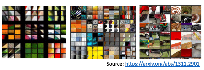
Intuitively, the pre-trained ResNet-152 model can be used as a feature extractor for images. We can inherit the properties of ResNet-152 through a technique called transfer learning. Transfer learning enables us to create a high-performing model with little data, computational resources, and in less time.

We’re going to take advantage of transfer learning. We do so by replacing the final pre-trained layer of the PyTorch ResNet-152 model with a new untrained extension of the model (which could simply be a single untrained layer). We then re-train this new model on the Zappos catalog while leaving the pre-trained layers immutable.

A dataset like Zappos50k, which has a single image of each of approximately fifty-thousand unique products will suffice for our example.

The Siamese network is trained on image pairings with target values where zero represents a pair of identical images, and values near and up to the value of one represent different images. In effect, the training process translates our images into a numerical encoding of features —referred to as feature vectors—and discovers a dimensional space where the distance between these vectors represents similarity. Details about the Siamese network are illustrated in the following diagram.

Ultimately, this model will provide us a means to measure the visual similarity between product images in the Zappos50k dataset.

This model yielded good results for this scenario, but you should always consider your options. For example, using triplet Loss, k-NN, or another clustering algorithm might be more suitable under certain circumstances. In the notebook that I’ve provided, I demonstrate an unconventional method that also yielded good results. The method is inspired by an DL technique called style transfer, which was first published in this research paper. The technique is generally used for artistic applications. For example, the technique could be used to synthesize an image of your home in the style of the artist Van Gogh by blending a photo of your home with Van Gogh’s Starry Night.

In the provided notebook, I demonstrate that the most important stylistic features of products in our catalog could be extracted through similar techniques to quantify the style of each product. In turn, we can then measure the stylistic similarity between products in our catalog. The technique didn’t require additional model training to produce better results than k-NN search (using the same model with L1 and L2 distance). It is purely an inference technique and can use user input to adapt to varying opinions in style in real time. See the notebook for great results even when using a simpler architecture like VGG-16 or ResNet-34 instead of ResNet-152. The following diagrams illustrate the concept.

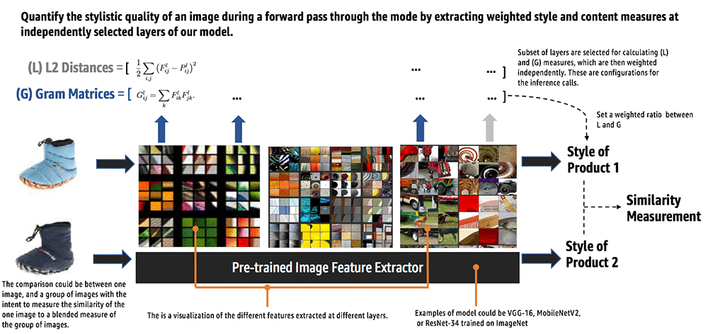
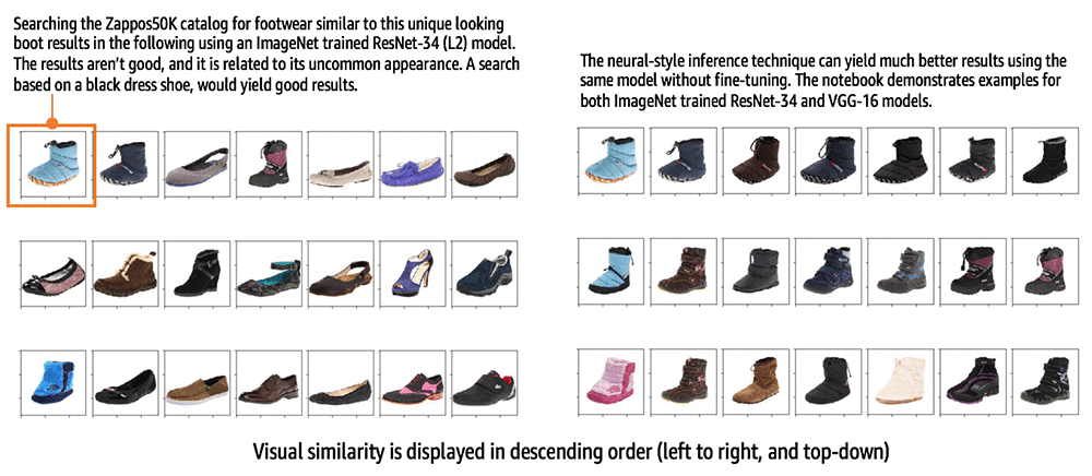
After we’ve defined the model architecture in PyTorch, a training job for our PyTorch model can be launched on a cluster of training servers managed by Amazon SageMaker with just a couple of lines of code using the AWS Python SDK. First, we create an Amazon SageMaker estimator object:

estimator = PyTorch(entry_point="siamese.py",
                    role=role,
                    framework_version='0.4.0',
                    train_instance_count=2,
                    train_instance_type="ml.p3.2xlarge",
                    source_dir=SOURCE_DIR,
                    hyperparameters=HYPERPARAMETERS)

The estimator contains information about the location of your PyTorch scripts, how to run them, and what infrastructure to use.

Next, we can launch the training job by calling the fit method with the location of your training data set in Amazon S3.

estimator.fit({'train':DATA_S3URI})

Behind the scenes, an Amazon SageMaker managed container for PyTorch is launched with the hardware specs, scripts, and data that were specified.

Model optimization

Depending on the infrastructure selected, we’ll have a good model in minutes to hours. However, we could further improve the performance of our model through a tedious process called hyperparameter tuning. We have the option of accelerating this process by leveraging Amazon SageMaker Automatic Model Tuning. This option is available to us regardless of which framework or algorithm we use.

First, we specify the hyperparameters and the range of values we want the tuning job to search over to discover an optimized model. See the following code snippet from the provided notebook. For our model, we explore a range of learning rates, different sizes for the final layer of our model, and a couple of different optimization algorithms.

HYPERPARAM_RANGES = {
                        'learning-rate': ContinuousParameter(1e-6, 1e-4),
                        'similarity-dims': CategoricalParameter([16,32,64,96,128]),
                        'optimizer': CategoricalParameter(['Adam','SGD'])
                    }

Second, we need to set an objective metric to define what we’re going to optimize. If your goal is to optimize a classification model, then your objective could be to improve classification accuracy. In this case, we’ve set the objective to minimize loss with this line of code in our notebook.

OBJECTIVE_METRIC_NAME = 'average training loss'

This minimizes the error between our model estimates, and the subjective truth of similarity measurements provided in the training data.

Next, we create a HyperparameterTuner by providing, as input, the PyTorch estimator (the one we created previously), the objective metric, hyperparameter ranges, and the maximum number of training jobs and degree of parallelism. This corresponds to the following code snippet in our notebook:

tuner = HyperparameterTuner(estimator=estimator,
                            objective_metric_name = OBJECTIVE_METRIC_NAME,
                            hyperparameter_ranges  = HYPERPARAM_RANGES,
                            metric_definitions = METRIC_DEFINITIONS,
                            max_jobs=2,
                            max_parallel_jobs=1)

Third, we launch the tuning job by calling the fit method:

tuner.fit({'train': DATA_S3URI})

The tuning job will launch training jobs according to your configurations, and proceed to find some optimal combination of hyperparameters using Bayesian optimization. This is an ML algorithm designed to accelerate the search for optimal hyperparameters. It’s better than common strategies like random or grid search. The intended benefit is to improve productivity through automation and lower the total training time required to produce an optimized model.

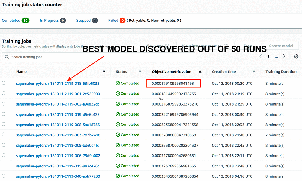
Generating product similarity scores

At the end of our tuning process, Amazon SageMaker delivers a well-tuned model that can be used to produce similarity scores. But we can get more value from our model if we could run graph queries on our similarity scores for analysis. We also need to deliver these queries with consistently low response times at scale to deliver a quality user experience on our customer-facing systems. Amazon Neptune makes this possible.

We’ll take the approach of pre-calculating and storing similarity scores in Amazon Neptune with the help of Amazon SageMaker Batch Transform. Batch Transform is well suited for high-throughput batch processing.

First, we ”bring our own” native PyTorch model serving script over to Amazon SageMaker. By doing so, we can run our script as a batch processing job at scale without having to build and manage the infrastructure. The provided model serving script illustrates a programmatic interface that you can optionally redefine (method override), as we did in our example. Each of the interface functions serves as a stage in a batch inference invocation.

• Model_fn(…): Loads the model into the PyTorch framework from the trained model artifacts.
• Input_fn(…): Performs transformations on the input batches.
• Predict_fn(…): Performs the prediction step logic.
• Output_fn(…): Performs transformations on predictions to produce results in the expected format.

Launching a batch transform job only requires a few configurations from the AWS Management Console, or a few lines of code using the AWS SDK. There are two distinct steps illustrated in our notebook. The first is model registration:

batchModel = PyTorchModel(model_data=MODELS_S3URI+'/model.tar.gz', 
                            role=role,
                            framework_version='0.4.0',
                            entry_point='batch.py',
                            source_dir=SOURCE_DIR)

batchModel.sagemaker_session = sagemaker_session
container_def = batchModel.prepare_container_def(instance_type=BATCH_INSTANCE_TYPE)
sagemaker_session.create_model(BATCH_MODEL_NAME, role, container_def)

After running this code, you should see your trained model listed in the Amazon SageMaker console.

At last, we launch the batch transform job, which could be done programmatically with another couple of lines of code:

from sagemaker.transformer import Transformer

transformer = Transformer(model_name=BATCH_MODEL_NAME,
                          instance_count=1,
                          instance_type= BATCH_INSTANCE_TYPE,
                          accept = 'text/csv',
                          output_path=BATCH_OUTPUT_S3URI
                         )

transformer.transform(BATCH_INPUT_S3URI, content_type= 'application/x-npy')

This code creates a Transformer object that is configured to use our trained model, our selected infrastructure, and an Amazon S3 location to write out the results of our job. When the transform method is executed, Amazon SageMaker provisions resources underneath the covers for you to perform the batch job. You can monitor the status of your job from the Amazon SageMaker console.

Transforming inference results to graph data

After our batch inference output is stored in Amazon S3, AWS Glue can run crawlers to automatically catalog this new dataset within our data lake. However, before we can load this data into Amazon Neptune, we need to transform our inference results into one of the supported open graph data formats. We’ll use the Gremlin compatible CSV format to keep our transformations simple. The format requires the graph to be formatted in two set of CSV files. One set defines the graph vertices (complete vertices file provided here), and another set defines the edges.

As a serverless ETL service, AWS Glue allows us to run Apache Spark jobs without managing any infrastructure. I can configure my transform job to run on a schedule, on demand, and optionally use Job Bookmarks for facilitating incremental reoccurring processing. This sample script demonstrates how our batch inference results can be transformed to graph edges compatible with Gremlin.

Let’s go to the AWS Glue console and kick off an AWS Glue job to perform this transformation.

AWS Glue allows us to specify the number of resources to allocate to our ETL job. Our dataset can be transformed in minutes while paying only for the resources used.

Loading our data into Amazon Neptune

Our dataset is now well suited for graph databases compatible with Gremlin and Apache TinkerPop, an open-source, vendor agnostic, graph computing framework. Thus, we have the freedom to move this data easily between a variety of graph databases. In our solution, we’ll use Amazon Neptune. By using an AWS managed database, we leave the bulk of the operational complexities, like reliability and scale, to AWS.

Amazon Neptune provides a RESTful API and a single command that we can execute from a terminal to bulk load our data. The provided prototype includes a Lambda function that demonstrates how to perform the bulk load in Python.

The provided prototype is intended as a sample. The sample data includes all 50K vertices corresponding to each product in the Zappos50K catalog. However, it only includes about 50M edges that represent the similarity scores between a subset of products. The full graph for the Zappos50K dataset would consist of over 1.2B edges. To handle that scale, you could be selective, and for instance, build a graph that only includes 10 edges per vertex to represent the top 10 most similar products to each item in the catalog.

Nonetheless, this approach isn’t necessary with Amazon Neptune. If there is value in storing the entire graph, Amazon Neptune can support this scale. Amazon Neptune is a purpose-built, high-performance graph database engine optimized for storing billions of relationships and querying the graph with milliseconds of latency. With support for up to 15 read replicas you can scale query throughput to hundreds of thousands of queries per second.

Explore the graph

After our data is in Amazon Neptune, we can interact with it through open tools like the Gremlin console. We can also query our data through various drivers supported through the Apache TinkerPop project. This Lambda function from our prototype uses the Gremlin language variant for Node.js. The sample function uses the Gremlin traversal language to query the most similar products to display for the selected product.

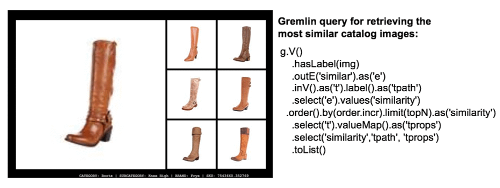
Amazon Neptune provides a high degree of durability by replicating our data six times across three Availability Zones at the storage layer. We have the option of adding up to 15 read replicas to improve the availability of our Amazon Neptune deployment. In the event the primary node fails, the database can fail over to any of our available replicas.

Furthermore, we can use our read replicas to serve queries. This provides us a means to scale our read workload or separate disparate workloads that would otherwise be inefficient to run together on the same node. For instance, we might have some heavy-duty graph traversal queries that we might want to run to support offline analysis. We would want to run these queries on a replica instead of our primary node.

The prototype has an example of a graph visualization page built on vis.js. You can tinker with this example, and create your own graph traversals and visualizations. This is an example of an offline workload that you could run on a replica to get some additional value from infrastructure that is otherwise mostly idle without introducing significant risk to the overall reliability of your database cluster.

Launching serverless microservices

There are many ways we can build out the rest of our web application on AWS to deliver a great experience. The fastest way, which allows us to spend more time on innovation, is to go serverless. We’ll use the standard serverless microservices architecture as presented in the AWS microservices whitepaper. Amazon API Gateway is used for API management, and AWS Lambda provides us with serverless compute.

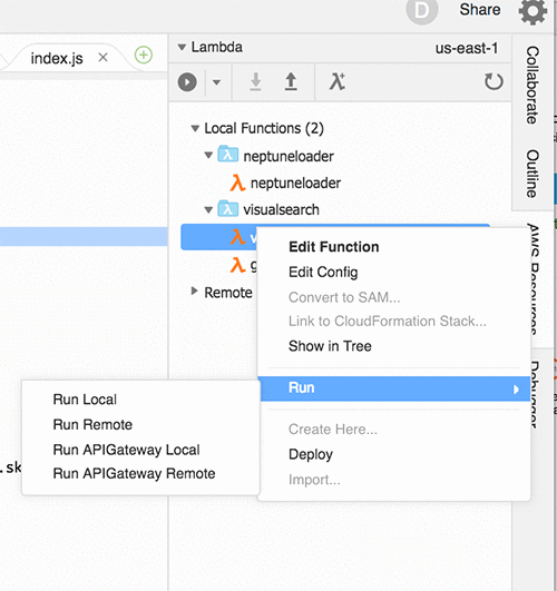
I prefer to use AWS Cloud9, a fully managed integrated development environment (IDE) to maximize development productivity when building AWS serverless applications. Within minutes, we can have a fully managed IDE instance pre-integrated for serverless development. The following picture illustrates the AWS Cloud9 native support for one-click serverless application deployments as well as for local and remote debugging for Amazon API Gateway and AWS Lambda.

Enhance the shop-by-style experience with minimal response times

We want to ensure our application provides a great customer experience by delivering the lowest possible response times. Since we expect our product catalog to be relatively static, we can cache our catalog along with our similarity measurements at the edge of the AWS network. We want to deliver our users a smooth shopping experience as they click through the different styles in our catalog. By caching everything at the edge of the AWS network, we can deliver web browser response times in 10s of milliseconds.

We can enable edge-caching in the Amazon API Gateway console by selecting a few check boxes. If the method you intend to enable caching on has query parameters like the one in our prototype, ensure that caching is selected on the appropriate parameters to ensure they’re accounted for in the cache key. The cache key determines how responses are uniquely cached.

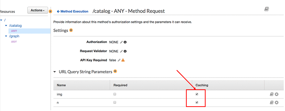
Select the Enable API cache check box in the appropriate API stage. In the following screenshot, I’ve enabled caching in my Prod stage, which represents the instance the API running in my production environment.

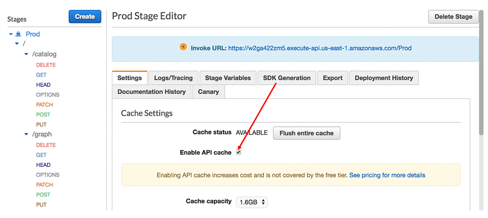
We should validate and monitor our API to ensure we continue to provide our customers with low response times by enabling AWS X-Ray. This requires enabling a single Amazon API Gateway configuration.

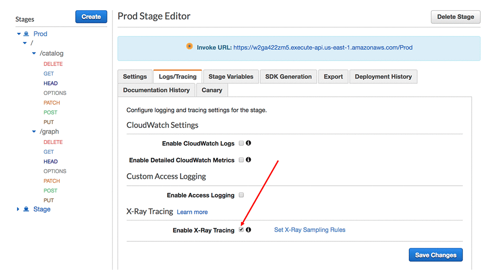
We can now observe the latency break down across the distributed components of our microservice through the AWS X-ray console service map. The diagram below illustrates response times for the prototype running in my AWS account once the edge-cache is enabled. The following diagram shows that the average response times for my deployment is within tens of milliseconds.

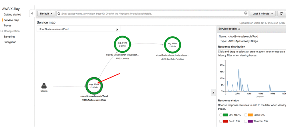
AWS X-Ray allows us to drill deeper into specific traces of our API calls. The specific API call that follows responded to a visual search query for products most similar to a particular Franco Sarto boot in our catalog within 4.0ms through the edge-cache.

Conclusion: Think big and build on

Together, we’ve created a unique, shop-by-style experience enabled by a tailor-made deep-learning model and a responsive web interface.  We’ve accomplished this in a short time and have taken advantage of the benefits of serverless.

The possibilities are limitless, and I hope you’re inspired to rethink the web experience. The journey doesn’t end with what we’ve created in this blog post. The customer experience can be further enhanced through voice-enabled interfaces and augmented reality. These technologies are within your reach on the AWS Cloud. Think big and build on!

About the Author

Dylan Tong is a Machine Learning Partner Solutions Architect at AWS. He works with technology and consulting partners to craft machine learning solutions, and develop their AI strategy through AWS AI.