Amazon SageMaker でセマンティックコンテンツレコメンドシステムを構築する

コンテンツレコメンドモデルをトレーニングしてデプロイする

このモジュールでは、組み込みの Amazon SageMaker k-Nearest Neighbors (k-NN) アルゴリズムを使用して、コンテンツレコメンドモデルをトレーニングします。

Amazon SageMaker K-Nearest Neighbors (k-NN) は、ノンパラメトリックなインデックスベースの教師あり学習アルゴリズムであり、分類および回帰タスクに使用できます。分類の場合、アルゴリズムはターゲットに最も近い k 個のポイントをクエリし、それらのクラスの最も頻繁に使用されるラベルを予測ラベルとして返します。回帰問題の場合、アルゴリズムは k 個の最近傍から返される予測値の平均を返します。

k-NN アルゴリズムを使用したトレーニングには、サンプリング、次元削減、インデックス作成の 3 つのステップがあります。サンプリングは、初期データセットのサイズを縮小して、メモリに収まるようにします。次元削減の場合、アルゴリズムはデータの特徴次元を削減して、メモリにおける k-NN モデルのフットプリントおよび推論のレイテンシーを削減します。次元削減の方法には、ランダム投影と高速 Johnson-Lindenstrauss 変換の 2 つの方法があります。通常、高次元 (d>1000) のデータセットには次元削減を使用して、次元の増加に伴いスパースになるデータの統計分析に支障をきたす「次元の呪い」を回避します。k-NN のトレーニングの主な目的は、インデックスを構築することです。インデックスを使用すると、値またはクラスラベルがまだ決定されていない点と、推論に使用する k 個の最も近い点の間の距離を効率的に検索できます。

次の手順では、トレーニングジョブの k-NN アルゴリズムを指定し、ハイパーパラメータ値を設定してモデルを調整し、モデルを実行します。次に、Amazon SageMaker が管理するエンドポイントにモデルをデプロイして予測を行います。

モジュールの所用時間: 20 分

ステップ 1:トレーニングジョブを作成して実行する
ステップ 1:トレーニングジョブを作成して実行する

前のモジュールでは、トピックベクトルを作成しました。このモジュールでは、トピックベクトルのインデックスを保持するコンテンツレコメンドモジュールを構築してデプロイします。

まず、シャッフルされたラベルをトレーニングデータの元のラベルにリンクする辞書を作成します。ノートブックで、以下のコードをコピーして貼り付け、[実行] を選択します。
```
labels = newidx 
labeldict = dict(zip(newidx,idx))
```
次に、次のコードを使用してトレーニングデータを S3 バケットに保存します。
```
import io
import sagemaker.amazon.common as smac


print('train_features shape = ', predictions.shape)
print('train_labels shape = ', labels.shape)
buf = io.BytesIO()
smac.write_numpy_to_dense_tensor(buf, predictions, labels)
buf.seek(0)

bucket = BUCKET
prefix = PREFIX
key = 'knn/train'
fname = os.path.join(prefix, key)
print(fname)
boto3.resource('s3').Bucket(bucket).Object(fname).upload_fileobj(buf)
s3_train_data = 's3://{}/{}/{}'.format(bucket, prefix, key)
print('uploaded training data location: {}'.format(s3_train_data))
```
次に、次のヘルパー関数を使用して、モジュール 3 で作成した NTM 推定器とよく似た k-NN 推定器を作成します。
```
def trained_estimator_from_hyperparams(s3_train_data, hyperparams, output_path, s3_test_data=None):
    """
    Create an Estimator from the given hyperparams, fit to training data, 
    and return a deployed predictor
    
    """
    # set up the estimator
    knn = sagemaker.estimator.Estimator(get_image_uri(boto3.Session().region_name, "knn"),
        get_execution_role(),
        train_instance_count=1,
        train_instance_type='ml.c4.xlarge',
        output_path=output_path,
        sagemaker_session=sagemaker.Session())
    knn.set_hyperparameters(**hyperparams)
    
    # train a model. fit_input contains the locations of the train and test data
    fit_input = {'train': s3_train_data}
    knn.fit(fit_input)
    return knn

hyperparams = {
    'feature_dim': predictions.shape[1],
    'k': NUM_NEIGHBORS,
    'sample_size': predictions.shape[0],
    'predictor_type': 'classifier' ,
    'index_metric':'COSINE'
}
output_path = 's3://' + bucket + '/' + prefix + '/knn/output'
knn_estimator = trained_estimator_from_hyperparams(s3_train_data, hyperparams, output_path)
```
トレーニングジョブの実行中に、ヘルパー関数のパラメータを詳しく見てください。

Amazon SageMaker k-NN アルゴリズムは、最近傍を計算するためのいくつかの異なる距離メトリクスを提供します。自然言語処理で使用される 1 つの一般的なメトリクスは、コサイン距離です。数学的には、2 つのベクトル A と B の間のコサイン「類似性」は、次の方程式で与えられます。

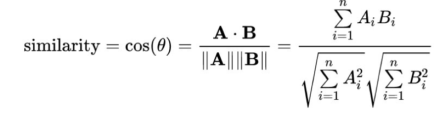
index_metric を COSINE に設定すると、Amazon SageMaker は自動的にコサイン類似度を使用して最近傍を計算します。デフォルトの距離は L2 ノルムで、これは標準のユークリッド距離です。公開時には、COSINE は faiss.IVFFlat インデックスタイプでのみサポートされ、faiss.IVFPQ インデックス方法ではサポートされないことに注意してください。

ターミナルに次のような出力が表示されます。
```
Completed - Training job completed
```
成功しました。このモデルは特定のテストトピックを与えられた最近傍を返すようにしたいので、ホストされたライブエンドポイントとしてデプロイする必要があります。

ステップ 2.コンテンツレコメンドモデルをデプロイする

NTM モデルで行ったように、k-NN モデルがエンドポイントを起動するための次のヘルパー関数を定義します。ヘルパー関数では、受け入れトークン applications/jsonlines; verbose=true は、k-NN モデルに、最近傍だけでなくすべてのコサイン距離を返すように指示します。レコメンドエンジンを構築するには、モデルによる上位 k 個の提案を取得する必要があります。これには、verbose パラメータをデフォルトの false ではなく true に設定する必要があります。

以下のコードをコピーしてノートブックに貼り付け、[実行] を選択します。

def predictor_from_estimator(knn_estimator, estimator_name, instance_type, endpoint_name=None): 
    knn_predictor = knn_estimator.deploy(initial_instance_count=1, instance_type=instance_type,
                                        endpoint_name=endpoint_name,
                                        accept="application/jsonlines; verbose=true")
    knn_predictor.content_type = 'text/csv'
    knn_predictor.serializer = csv_serializer
    knn_predictor.deserializer = json_deserializer
    return knn_predictor
import time

instance_type = 'ml.m4.xlarge'
model_name = 'knn_%s'% instance_type
endpoint_name = 'knn-ml-m4-xlarge-%s'% (str(time.time()).replace('.','-'))
print('setting up the endpoint..')
knn_predictor = predictor_from_estimator(knn_estimator, model_name, instance_type, endpoint_name=endpoint_name)

次に、推論を実行できるようにテストデータを前処理します。

以下のコードをコピーしてノートブックに貼り付け、[実行] を選択します。

def preprocess_input(text):
    text = strip_newsgroup_header(text)
    text = strip_newsgroup_quoting(text)
    text = strip_newsgroup_footer(text)
    return text    
    
test_data_prep = []
for i in range(len(newsgroups_test)):
    test_data_prep.append(preprocess_input(newsgroups_test[i]))
test_vectors = vectorizer.fit_transform(test_data_prep)

test_vectors = np.array(test_vectors.todense())
test_topics = []
for vec in test_vectors:
    test_result = ntm_predictor.predict(vec)
    test_topics.append(test_result['predictions'][0]['topic_weights'])

topic_predictions = []
for topic in test_topics:
    result = knn_predictor.predict(topic)
    cur_predictions = np.array([int(result['labels'][i]) for i in range(len(result['labels']))])
    topic_predictions.append(cur_predictions[::-1][:10])

このモジュールの最後のステップでは、コンテンツレコメンドモデルを探索します。

ステップ 3.コンテンツレコメンドモデルを探索する
ステップ 3.コンテンツレコメンドモデルを探索する

予測を取得したので、k-NN モデルでレコメンドされる最も近い k 個のトピックと比較して、テストトピックのトピック分布をプロットできます。

以下のコードをコピーしてノートブックに貼り付け、[実行] を選択します。
```
# set your own k.
def plot_topic_distribution(topic_num, k = 5):
    
    closest_topics = [predictions[labeldict[x]] for x in topic_predictions[topic_num][:k]]
    closest_topics.append(np.array(test_topics[topic_num]))
    closest_topics = np.array(closest_topics)
    df = pd.DataFrame(closest_topics.T)
    df.rename(columns ={k:"Test Document Distribution"}, inplace=True)
    fs = 12
    df.plot(kind='bar', figsize=(16,4), fontsize=fs)
    plt.ylabel('Topic assignment', fontsize=fs+2)
    plt.xlabel('Topic ID', fontsize=fs+2)
    plt.show()
```
次のコードを実行して、トピック分布をプロットします。
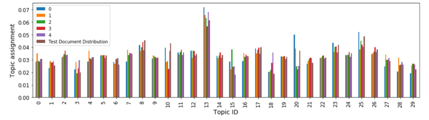
```
plot_topic_distribution(18)
```
ここで、他のトピックをいくつか試してみましょう。次のコードセルを実行します。
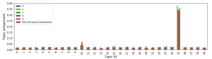
```
plot_topic_distribution(25)
```
```
plot_topic_distribution(5000)
```
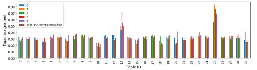
選択したトピックの数 (NUM_TOPICS) によっては、プロットが多少異なる場合があります。しかし、全体として、これらのプロットは、k-NN モデルによるコサイン類似度を使用して検出された最近傍ドキュメントのトピック分布が、モデルに入力したテストドキュメントのトピック分布とかなり類似していることを示しています。

結果は、最初にドキュメントをトピックベクトルに埋め込み、次に k-NN モデルを使用してレコメンデーションを提供することにより、セマンティックベースの情報検索システムを構築する方法として k-NN が優れている可能性があることを示唆しています。